Preference Mapping in Excel tutorial

This tutorial helps you understand the concept of preference mapping, draw a preference map and interpret it in Excel using XLSTAT.

What is Preference Mapping?

This tutorial was inspired by [Schlich P, McEwan J.A. (1992). Cartographie des Préférences. Un outil statistique pour l'industrie agro-alimentaire. Sciences des aliments, 12, pp 339-355] and by exchanges between the Addinsoft development team and some experts of sensory data analysis.

We distinguish two types of Preference Mapping methods:

1. Internal Preference Mapping

This method corresponds to MDPREF (Multidimensional Analysis of Preference Data) and is based on a PCA (Principal Component Analysis) performed on preference data with products in rows (observations) and consumers in columns (variables). The data are ratings given by the consumers for each product. The preference map is the biplot (two or three dimensional) of the observations and the variables.

As the capacity to summarize of the preference map diminishes with the number of consumers (the number of axes to interpret increases), a non-metric PCA is sometimes used to reduce the number of necessary axes. The non-metric PCA consists of a monotone transform of the data so that the variability explained by the k (k=2 or 3) first axes is maximized. This transform implies that we consider the ratings have an ordinal meaning, and that the distances or ratios between the ratings are not important. To reduce the number of axes you might also want to group the consumers and to perform the PCA with the groups as variables.

Internal preference mapping allows to generate a map on which one can identify the consumers' or groups of consumers preferences represented as vectors.

2. External Preference Mapping

This method allows to relate the preferences shown by the consumers to some physico-chemical, sensory or economical characteristics of the products. This approach is essential as it gives a reliable basis to the marketing and R&D teams for adapting or creating products that will correspond to the consumers' expectations.

This method requires an additional table that describes the products with a series of criteria. Contrary to what is done with internal preference mapping, the first step consists in mapping the products on the basis of their characteristics.

This can be obtained by running a Principal Component Analysis (PCA), a Correspondence Analysis (CA) or a Generalized Procrustes Analysis (GPA).

This first visualization is named sensory map. By applying the PREFMAP method, we then model for each consumer (or group of consumers) the ratings that have been given to the products, using as explanatory variables the characteristics of the products, with the aim of representing the consumers on the sensory map. The full model writes:

Y = Si aiXi + Si biXi’² + Sij cijXiXj

The PREFMAP method uses four sub-models:

• Vector model: bi and cij are null. The model is a hyperplan. This model allows to display the observations on a sensory map as vectors. The size of the vectors can be related to the R’² of the model; in that case the longer the vector, the better the underlying model. The consumer's preference increases the further you go in the direction of the vector. Interpreting the preference can be done by projecting the products on the various vectors (product preference). The drawback of that model is that it neglects that for some criteria such as saltiness or temperature, the preference can increase until an optimal value, and then decrease;

• Circular ideal point model: The bi are equal and the cij are null. The model corresponds to a hyperquadric hypersurface. If the surface has a maximum in terms of preference we will talk of an ideal point. If this surface has a minimum we will talk of anti-ideal point. With the circular model it is possible to trace isopreference circular lines around the ideal or anti-ideal point.

• Elliptical ideal point model: The cij are null. The model corresponds to a hyperquadric hypersurface. In this case the isopreference lines are ellipses, which make the interpretation of the distances of the products to the ideal or anti-ideal points more complex. If the bi have opposite signs, there is no ideal or anti-ideal point but only a saddle point which interpretation is tricky.

• Quadratic surface model: This model corresponds to the complete model which shape is a hypersurface. This model allows to take into account interactions between the characteristics (the cijXiXj).

How do I run Preference Mapping with XLSTAT?

The following example shows how one can create a preference map using the PREFMAP method.

• The consumer acceptability data: 99 consumers rated 10 different commercial samples of potato crisps. These data have been obtained from the article by Schlich and McEwan (1992). The ratings have been descritized from 1 to 30 (30 corresponds to the highest acceptability). These data are stored in a 99 x 10 table.

• The average ratings computed from the ratings given by 8 experts to the 10 crisps samples for 4 texture attributes and 7 flavor attributes. These data, simulated for the purpose of teaching by the author of this tutorial on the basis of the article by Schlich and McEwan (1992), make up a 10 x 11 table.

Step 1: Grouping the consumers

Our focus is on the ratings given by the 99 consumers. As the number of consumers is significant, we decided to group them into homogeneous groups in order to make the PREFMAP results easier to interpret. We chose the Agglomerative Hierarchical Clustering (AHC). As a tutorial on AHC already exists, we do not elaborate on that subject here. The dialog box of the AHC has been filled in as shown below.

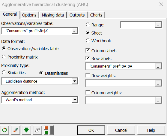
In the Options tab, the "Center / Reduce" option applied to "Rows" has been activated in order to diminish the differences between the judgment scales of the consumers. The truncation option was not activated.

By looking at the dendrogram, it makes sense to decide to work with 9 groups.

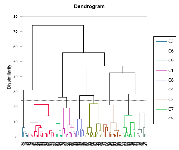
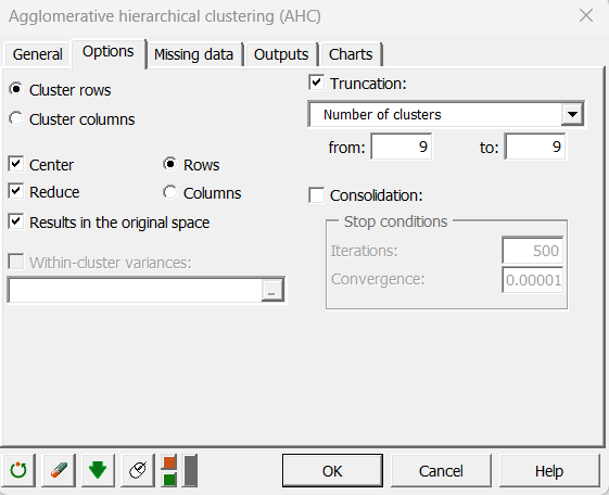
We then re-run the AHC while specifying that we request 9 clusters. The dialog box has been filled in as displayed below. The only difference with the previous case is that we ask for a truncation.

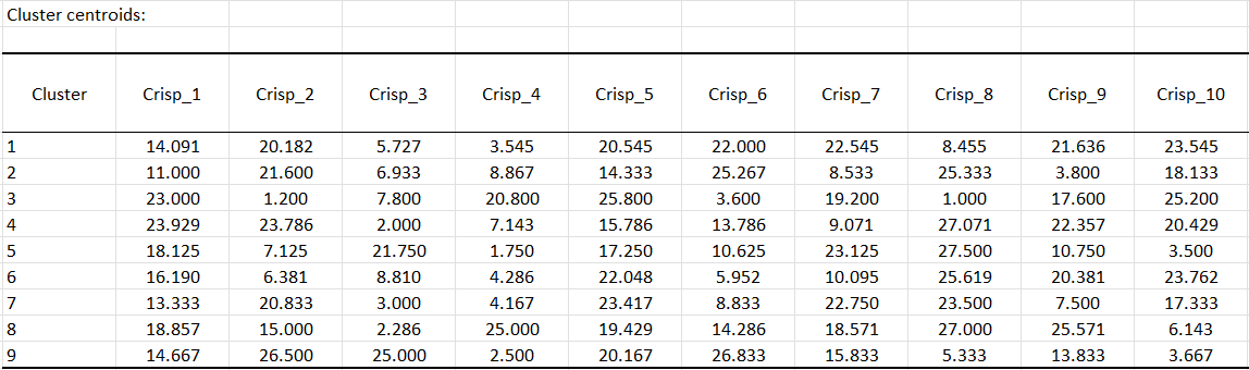
We then store the centroids of the clusters for the last step of the analysis. The table is copied and paste (Edit / Paste special with Transposed option) in a new sheet named "Clusters' pref.".

Step 2: Creating the preference map using the PREFMAP method

In this section we apply the PREFMAP method, using the scores given by the experts and the ratings given by the consumers summarized by the standardized ratings for the 9 clusters.

Setting up a preference mapping

To activate the Preference Mapping dialog box, start XLSTAT, then select the Sensory data analysis menu and then the Preference Mapping feature:

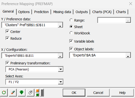
When you click on the button, the Preference Mapping dialog box will appear. Select the data on the Excel sheet. To the "Y / Preference data" correspond the ratings of the 8 clusters. The "X / Configuration" corresponds to scores given by the experts. The "preliminary transformation" option allows to directly do a PCA on the raw data. We selected the Pearson Method.

In the Options tab to select the best model among the four possible models, we used an F-ratio test, with a 0.1 (10%) significance level. That means that if a more complex model does not give an F-ratio with a p-value lower than 0.1 the more complex model is rejected.

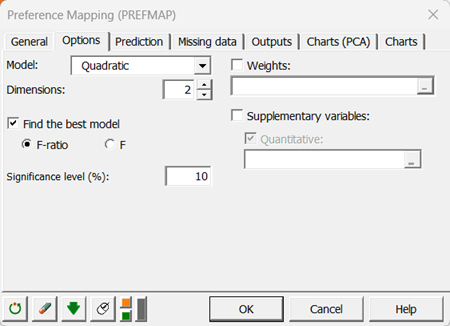
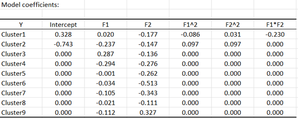
We selected the coefficients of the model to determine the length of the vectors on the preference map.

Interpreting a preference mapping

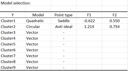
The results we obtain (see below) show that the vector model is the best model for the clusters 3 to 9. For cluster 1 the quadratic model performs best. However, it is not significant. The circular model is the best model for cluster 2 and it is significant. For the quadratic model retained for cluster 1, we do not have an ideal point but a saddle point. The saddle point represents a threshold where the variability of the preference is low, before increasing (or decreasing in the opposite direction) quicker. For cluster 2 we have an anti-ideal point. The anti-ideal point corresponds to the lowest preference for the group.

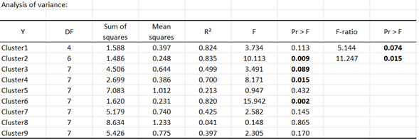
Looking at the analysis of variance table we see that the models are significant only for clusters 2, 3, 4 and 6.

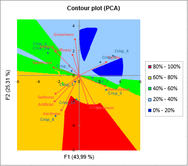
The preference map allows to quickly interpret the results. When looking at both the preference map and the correlations circle of the PCA, we see that the consumers of cluster 3 prefer chips that are not melting, but not too overcooked and crispy. Consumers from cluster 6 like crispy chips and dislike greasy chips. For cluster 2 it is hard to know what they prefer, but it seems that they strongly dislike (anti-ideal point) a chip that would be salty and average for all the criteria (the point is close to the origin).

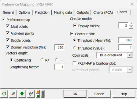
Note: If an ideal/anti-ideal/saddle point is not displayed because out of the plotting area, to extend the mapping area, you can increase the value of the "Domain restriction" in the "Charts" tab of the dialog box.

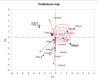
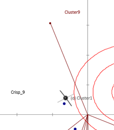
If we zoom on the cluster to which corresponds an anti-ideal point, you can see that a grey cross is displayed. The thicker lines corresponds to the direction in which the preference increases, and the thinner ones to the direction in which it diminishes. The longer the line, the stronger the effect.

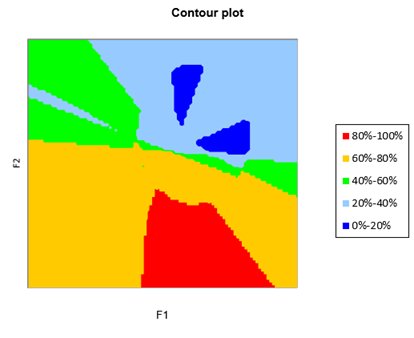
The contour plot allows to see how many clusters have a preference above average in a given region of the preference map (this is determined using all the fitted models).

Both maps can be superimposed. To do that, select the PREFMAP & Contour plot option on the Charts dialog box.

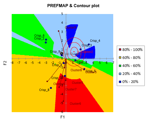
The preference orders for the various groups of consumers are displayed.

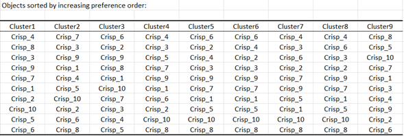
We notice that the crisp 4, characterized by an earthy, not sweet and not salty taste, is not liked at all by clusters 1, 4, 6, 7 and 8. Crisps 8 are the preferred ones for most clusters, except by cluster 9. The marketing and R&D teams will be able to take this information into account to direct their creation of new crisps towards the right directions.