Holt-Winters seasonal multiplicative model in Excel
This tutorial will help you set up and interpret a Holt-Winters seasonal multiplicative model to smooth a time series in Excel using XLSTAT.
Dataset to fit a Holt-Winters seasonal multiplicative model to a time series
The data have been obtained in [Box, G.E.P. and Jenkins, G.M. (1976). Time Series Analysis: Forecasting and Control. Holden-Day, San Francisco], and correspond to monthly international airline passengers (in thousands) from January 1949 to December 1960.

We notice that on the chart, there is global upward trend, that every year, a similar cycle starts while the variability within a year seems to increase over time. The Holt-Winters seasonal multiplicative model is well adapted for this type of time series.
Setting up a Holt-Winters seasonal multiplicative model to a time series
After opening XLSTAT, select the XLSTAT / Time / Smoothing command.

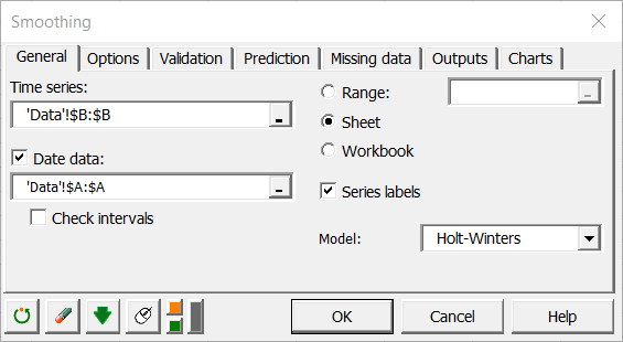
Once you've clicked on the button, the Smoothing dialog box will appear. Select the data on the Excel sheet.
The Series to analyze corresponds to the series of interest, the "Passengers".
After you selected the data, select the Holt-Winters method.
The option Series labels is activated because the first row of the selected data contains the header of the variable.
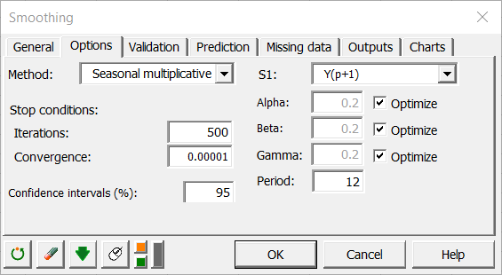
In the options tab, select the seasonal multiplicative sub-method.
Then, so that the model parameters are optimized (ordinary least square), check the optimized option. The period of the series is set to 12, because it seems the cycles are repeated every year (12 months).
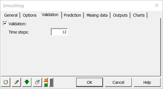
Last, in the validation tab, enter 12 so that the last 12 values are not used to fit the model, but only to validate the model.
The computations begin once you have clicked on OK. The results will then be displayed.
Results of the fitting of a Holt-Winters seasonal multiplicative model to a time series
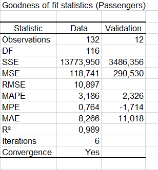
The first table displays the various criteria that allow to evaluate the quality of the fit, and to compare the fit of this model with other models (if available). We notice here that the R’² is very close to one, which indicates a very good fit.
Below the table that displays the estimates of the parameters of the model, a table gives the values of the original series, and the smoothed series (the predictions). Because of the constraints of the model, predictions are not available for the 13 first observations. Notice that a time variable "T" has been created to facilitate the graphical representation. For the last 12 observations predictions have been computed in validation mode and a confidence range is available.

On the chart below, we can visually see that the predictions are very close to the data.

In order to analyze better the results for the 12 validation months, we have zoomed on the 24 last months.

We notice that the quality of the previsions is excellent. Only twice, at T=135 and T=140 (March 1960 and August 1960), the model overestimates the reality by respectively 10% and 5%. As a conclusion, the Holt-Winters seasonal multiplicative model allows to very well take into account the upward trend, the seasonalities and the increase in variability within a period.
Was this article useful?
- Yes
- No