Using differencing to obtain a stationary time series
This tutorial will help you describe a time series and transform it so that it becomes stationary, in Excel using the XLSTAT software.
Dataset for the descriptive analysis and transformation of time series
The dataset has been obtained in [Box, G.E.P. and Jenkins, G.M. (1976). Time Series Analysis: Forecasting and Control. Holden-Day, San Francisco], and corresponds to monthly international airline passengers (in thousands) from January 1949 to December 1960. It is widely used as a nonstationary seasonal time series
The goal of this tutorial is to show how helpful a descriptive analysis can be prior to a modeling approach.
 We notice a global upward trend on the chart. Every year, a similar cycle starts while the variability within a year seems to increase over time. In order to confirm this trend we are going to analyze the autocorrelation function of the series.
Descriptive analysis of a time series
Setting up a descriptive analysis of time series with XLSTAT
-
Open XLSTAT
-
Select the Advanced features / Time series analysis / descriptive analysis menu. The Descriptive analysis dialog box will appear.
-
In the General tab, select the values of the time series.

-
In the Options tab, check the Automatic option in order to choose an automatic number of time steps. Set the confidence intervals to 95% and check the white noise tests option
-
In the Outputs tab, make sure the Autocorrelations and Partial autocorrelations options are checked
-
In the Charts tab, check Autocorrelogram and Partial autocorrelogram.
How to interpret the descriptive statistics of a time series?
The first table displays the summary statistics. Then the Normality test and white noise tests table are displayed. The Jarque-Bera test is a normality test, based on the skewness and kurtosis coefficients. The higher the value of the Chi-square statistic, the more unlikely the null hypothesis that the data are normally distributed. Here the p-value, which corresponds to the probability of being wrong when rejecting the null hypothesis, is close to 0.012. With an alpha=0.05 significance level, one should reject the null hypothesis.
The three other tests (Box-Pierce, Ljung-Box, McLeod-Li) are computed at different time lags. They allow us to test whether the data can be assumed to be white noise. These tests are also based on the Chi-square distribution. They all agree that the data cannot be assumed to be generated by a white noise process. While the sorting of the data has no influence on the Jarque-Bera test, it does have an influence on the three other tests which are particularly suited for time series analysis.

Below the table that displays the descriptive functions of the time series, two bar charts show the evolution of the autocorrelation function (ACF) and of the partial autocorrelation function (PACF). The 95% confidence intervals are also displayed. By looking at the autocorrelogram, we can identify an evident lag 1 autocorrelation, as well as a seasonality that seems to be of 12 months.

Transformation of a time series
In order to improve the normality of the data, we want to perform two transformations:
First, we want to stabilize the increasing variability of the series. Second, we want to remove the autocorrelations by differencing the series.
Setting up the transformation of a time series with XLSTAT
-
Select the Advanced features / Time series analysis / Time Series Transformation menu. The Descriptive analysis dialog box will appear.
-
In the General tab, select the values of the time series.
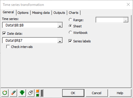
-
In the Options tab, check the Box-Cox option and fix the lambda parameter to 0 in order to perform a log transformation of the series. The log transformation is often a good choice for removing increasing variability.
Results of the log transformation
We first see a table and two charts: one for the original data and the other for the log-transformed series. As expected, the transformation has removed the increasing variability.

Setting up a differencing transformation with XLSTAT
-
Select the Advanced features / Time series analysis / Time Series Transformation menu. The Descriptive analysis dialog box will appear.
-
In the General tab, select the values of the log-transformed time series.
-
In the Options tab, check the differencing option and set the d value to 1 to remove the trend, D to 1, and s to 12 to remove the 12-month seasonal component.
Results of the differencing transformation
The resulting chart shows that the differencing transformation effectively removed the trend.

Running a similar descriptive analysis on our transformed time series gives us the following results.
The Jarque-Bera test confirms that the series gets closer to a normal sample (we went from 0.012 to 0.027) but remains not stationary as confirmed by the white noise tests.

Transformations have not been efficient enough. Indeed, the autocorrelogram indicates that some significant component remains at lag 1 and 12. Further investigations are needed in order to understand the underlying phenomenon.

Setting up a seasonal decomposition of the time series
-
Select the Advanced features / Time series analysis / Time Series Transformation menu. The Descriptive analysis dialog box will appear.
-
In the General tab, select the values of the transformed time series.
-
In the Options tab, check the seasonal decomposition option and select the multiplicative model, which seems appropriate as the time series exhibits a clear multiplicative behavior on the natural scale. The period is set to 12 for a 1-year periodicity on monthly data.
Results of the seasonal decomposition of the time series
Once computed, the decomposition is displayed via 4 plots: the original series, a trend component, a seasonal component, and a random component. The last 3 series can be multiplied by each other in order to reconstruct the original series.

The stationarity of the random component might be tested now. However, we may first transform again this Random component using the log transformation so that it is centered on 0.

The descriptive analysis is launched again in this series. This time the Jarque-Bera test does not allow to reject the hypothesis of a normally distributed variable.

Unfortunately, a seasonal pattern, less significant than before, remains visible in the autocorrelogram plot. This would call again for some further work to identify the generating process.
Was this article useful?
- Yes
- No