Cointegration test on time series in Excel tutorial
This tutorial will help you set up and interpret cointegration tests on time series in Excel using the XLSTAT statistical software.
Dataset for running a cointegration test
This tutorial uses a dataset extracted from the database made available by the Bank of England. It is made of two time series:
-The monthly average 12 month Forward exchange rate of US$ into Sterling labeled XUMADSY,
-The monthly average Spot exchange rate US$ into Sterling labeled XUMAUSS.
Both series cover a time period ranging from January 1979 to December 1999.
Goal of this tutorial
The exchange rate expresses the price of one currency, the foreign one, in terms of another, the domestic one. In our tutorial, we will be considering the 12 month Forward and the Spot exchange rates of the US dollar in terms of the British Pound over the period 1979-1999. On the one hand, the 12 month forward exchange rate is a hedging contract in which two parties agree at present time upon the rate at which they will exchange the two currencies in the future (12 months ahead). On the other hand, the Spot exchange rate sets the present relative value of the two currencies.
In the context of the Covered Interest Parity (CIP), the log of the Spot and Forward exchange rates is expected to be related to the foreign to domestic differential of interest rates by the following relation:
lnForward - lnSpot = rDiff. where lnForward is the log of the Forward exchange rate, lnSpot is the log of the Spot exchange rate and rDiff is the differential interest rate.
Under the hypothesis of efficient financial markets, a situation of risk-less profit where one would borrow into a foreign currency, invest at risk-free rate in this currency and lock its selling price into domestic currency in a forward sale should not be possible. As a consequence, the interest rate differential is expected to be I(0) (or stationary). As it is generally accepted in the international finance literature that both the Spot and Forward exchange rates are integrated of order 1 (noted or I(1)), a cointegration relationship should exist between the log Spot and Forward exchange rates for the CIP relationship stated above to hold.
In the following tutorial, we should first transform our time series and test their I(1) status. Then, we should assess that those two I(1) processes can combine to a I(0) process, in other words that the two time series are cointegrated, by the mean of a cointegration test following Johansen's approach.
Transformation of time series
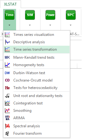
First, we have to transform the series extracted from the database of the Bank of England to obtain their log values. After opening XLSTAT, select Time / Time series transformation (see below).
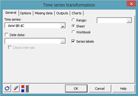
 The Time series transformation dialog box appears as shown below. Select the Time series on the Excel sheet.
The option Series labels is activated because the first row of the selected data contains the headers of the variables.
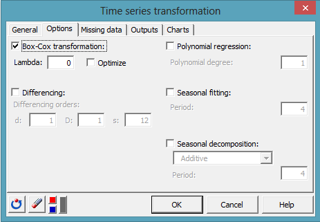
 In the Options tab, select Box-Cox transformation and set the value of Lambda to 0 to apply a log transformation to the series:
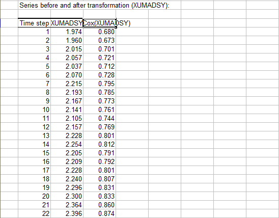
 Once you click on OK, the computations are performed and the two transformed series are displayed on a new sheet.
First the 12 month Forward exchange rate (XUMADSY) and its log transformation (Box-Cox(XUMADSY)):
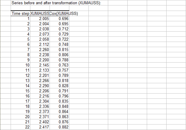
 Followed by the Spot exchange rate (XUMAUSS) and its log transformation (Box-Cox(XUMAUSS)):
Descriptive analysis
Now that our time series are ready, we should apply a descriptive analysis on them in order to control that they present the expected characteristics.
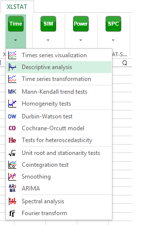
To perform a descriptive analysis, click on Time / Descriptive analysis as shown below.
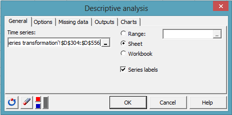
 Select the two transformed series, Box-Cox(XUMADSY) and Box-Cox(XUMAUSS), with the help of the Ctrl key to select multiple fields:
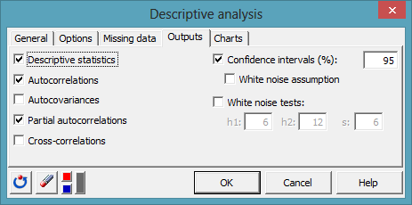
 In the Outputs tab, make sure the Autocorrelations and the Partial Autocorrelations options are activated as shown below.
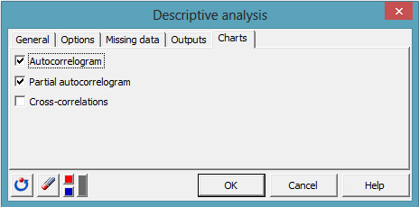
 In the Charts tab, activate the Autocorrelogram (ACF) and Partial Autocorrelogram (PACF) options:
 Once you clicked on OK, the descriptive statistics as well as the ACF and PACF are displayed for the two series.
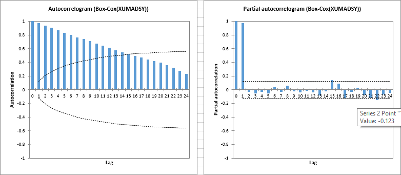
First, as shown below, the ACF of the Box-Cox(XUMADSY) series exhibits a large number of significant lags.
Looking at the PACF, it seems that those high order correlations are explained mainly by the 1 lag autocorrelation as it is the only one strongly significant in the PACF.
This behavior is quite compatible with the expected I(1) time series.
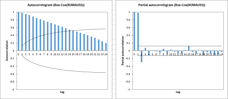
The situation is highly similar for the second time series named Box-Cox(XUMAUSS) as shown below with a strongly significant lag-1 in the PACF.
Unit root tests
After those preliminary checks, we are ready to test the I(1) aspect of our time series. We will apply two unit root tests on our transformed time series: a Dickey-Fuller test (DF) and a Phillips-Perron test (PP).
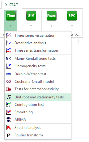
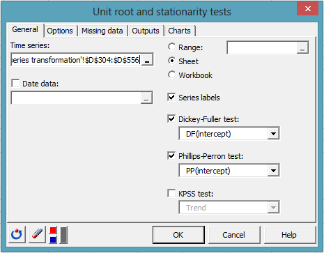
Select Time / Unit root and stationarity tests as shown below.
 In the time series field, select the two transformed series, Box-Cox(XUMADSY) and Box-Cox(XUMAUSS), and activate the Dickey-Fuller and thePhillips-Perron tests as shown below.
Regarding the model selection, the model with an intercept is the one that best describes our data. You should therefore select the intercept option for both the DF and PP tests.
Once you have clicked on OK, the tests are performed and the results are displayed for the two series.
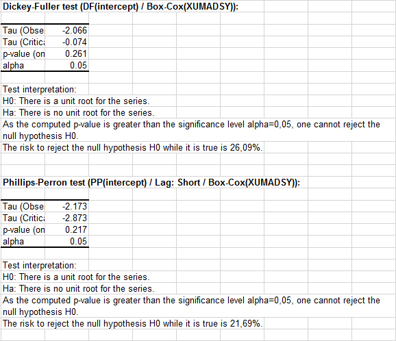
For the Box-Cox(XUMADSY) series, neither the DF nor the PP test reject the null hypothesis of a presence of a unit root in the data generating process (see below).
 For the second series, the confidence level that one should not reject the null hypothesis is even stronger:
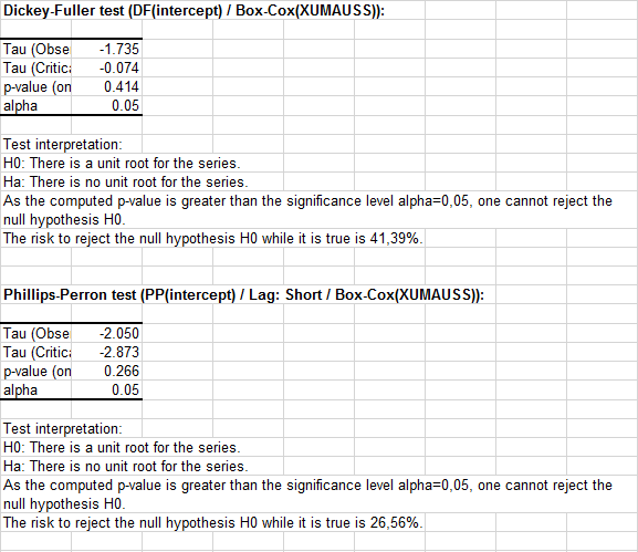 To conclude on this part, it seems that the log of the Forward and Spot exchange rates are both I(1). This is in agreement with what is expected from the economic theory.
We should now check that a linear relationship between those two I(1) series that produces an I(0) series exists.
Setting up a cointegration test
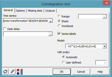
To test the existence of this relationship, we will perform a cointegration test following Johansen's approach. Click on Time / Cointegration test:
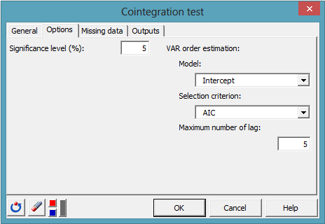
 The Cointegration test dialog box appears as shown below. First, select our two transformed time series, Box-Cox(XUMADSY) and Box-Cox(XUMAUSS). Then, we must select a model for the test.
Both series have non zero means with no drift and the cointegration relationship as stated at the beginning of this tutorial is not expected to have a linear trend. Therefore the H1* restriction seems suitable for our test.
Finally, we don't know about the VAR order that best apply to our group of series. We will then let XLSTAT estimate its value by selecting the Automatic option as shown below.
 In the Options tab, we must select a model and a criterion for the VAR order estimation. Again a model with intercept seems appropriate and we will use the AIC criterion:
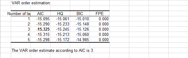
Click on OK and the Johansen's cointegration test is performed. The first table (see below) displays the result for the VAR order estimation. In bold, the minimum AIC value gives a VAR order of 3 or VAR(3) for our system which means 2 lags in difference for the Vector Error Correction Model (VECM). We can check that there is a good agreement between the four criteria.
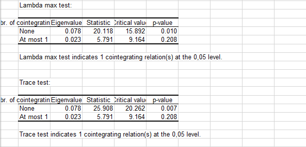
 Then the results for both tests, the max eigen test (or lambda test) and the trace test are displayed (see below). Both tests agree on the rank(1) of cointegration of the system or equivalently on the existence of 1 cointegrating relationship between the two series. P-values and critical values for both tests are estimated using the surface regression approach described in MacKinnon-Haug-Mechelis(1998).
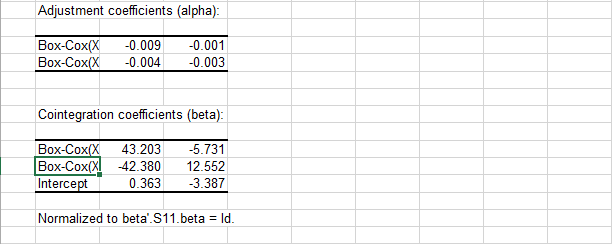
 Finally, the factorization of the cointegrating matrix is given in the form of the impact matrix (alpha) and the cointegration coefficients (beta) following the normalization proposed by Johansen:
Conclusion
We have been able to transform the two time series and perform subsequent tests to validate the hypothesis of two I(1) series.
Then, we performed a cointegration test following Johansen's approach that lead us to conclude that 1 cointegrating relationship might exist between the two series.
Therefore, for the time period running from 1979 to 1999, the log 12 month Forward and log Spot exchange rates series of US$ into Sterling exhibit one cointegrating relationship as expected by the Covered Interest Parity hypothesis. Now, you should try your own analysis using another dataset. What about the same dataset but up to the present days? This might lead to some surprising results.
Was this article useful?
- Yes
- No