Redundancy Analysis (RDA) in Excel tutorial

This tutorial will help you set up and interpret a Redundancy Analysis or RDA in Excel using the XLSTAT statistical software.

What is Redundancy Analysis?

Redundancy Analysis (RDA) can be thought of as a multivariate approach of linear models, which means a linear model with many dependent variables. RDA works by building a Principal Component Analysis (PCA) on the response variables (Y matrix) under the constraint that the produced axes – the canonical axes – are also a linear combination of the explanatory variables (X matrix). RDA is often used in ecology to explain a matrix of sites / species abundances by a set of environmental variables that often capture gradients (ranges of temperatures or soil depths or soil nutrient contents…). In a RDA context, relationships between the Y and X variables are assumed to be linear.

What is the difference between Redundancy Analysis and Canonical Correspondence Analysis?

Canonical Correspondence Analysis (CCA)is a method related to Redundancy Analysis. While in RDA we assume that the relationships between the Y and X matrices are linear, in CCA we assume that they are unimodal. In ecology, CCA is closer to the concept of species niche for which environmental gradients should be sampled at their entire scales for the analysis. RDA may be more adapted in cases where smaller parts of environmental gradients are captured.

What are conditioning variables and what is partial RDA?

Similar to Canonical Correspondence Analysis (CCA), RDA includes the possibility of removing the effect of undesired constraining X variables in order to focus the attention on effects of interest. Undesired variables include block effects or any other environmental constraint that may hide the effects of explanatory variables relevant to the question under investigation. This produces what we call a partial RDA (or partial CCA in the case of CCA). Undesired variables are called conditioning variables. XLSTAT allows for the selection of conditioning variables both in RDA and CCA under the General tab in the features dialog boxes (activate Partial CCA or Partial RDA).

Dataset for this tutorial on Redundancy Analysis in Excel

The data corresponds to the abundances of 30 plant species (in columns) at 20 sites (in rows) in a dune environment. Species names are the combinations of the first 4 letters of their genus and the first four letters of their species names in Latin. Sites are also described by two environmental variables in columns: - Soil thickness: quantitative variable, depth of the A1 soil horizon.

• Management: qualitative variable with levels BF (Biological farming), HF (Hobby farming), NM (Nature Conservation Management) and SF (Standard Farming).

The data are extracted from [Jongman, R.H.G, ter Braak, C.J.F & van Tongeren, O.F.R. (1987). Data Analysis in Community and Landscape Ecology. Pudoc, Wageningen]. Other environmental variables from the same data source have been excluded for this tutorial.

Goal of this tutorial on Redundancy Analysis

The goal of this tutorial is to investigate the linear relationships between management type and A1 soil horizon depth on dune plant communities using Redundancy Analysis.

Setting up a Redundancy Analysis in XLSTAT

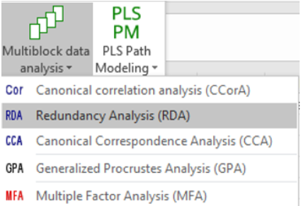
After opening XLSTAT, select the Advanced Features / Multiblock Data Analysis / Redundancy Analysis command: Select the Site / Species matrix in the Response Variables field. Under Explanatory Variables, select Soil Thickness in the Quantitative field and Management type in the Qualitative field. In the Options tab, activate the Permutation test option, and set the number of permutations to 1000. If your response variables or your quantitative explanatory variables are not on the same scale, consider activating the Reduce options for the corresponding matrix. In the Charts tab, deactivate the Observations option under Display.

Click on OK. The computations are launched and the results displayed in a new spreadsheet.

Interpreting the outputs of a Redundancy Analysis

One first dialog box pops up allowing you to select the axes to represent in the RDA charts. With axes F1 & F2, we are able to represent 80% of the constrained inertia (explanation further below). Select those two axes and click Done. After descriptive statistics on both the response and the explanatory variables, the Inertia summary table appears: Here we are investigating the inertia or variability of the response variables. It is split into: - Constrained inertia, which is the part that is explained by the explanatory variables matrix.

• Unconstrained inertia, which is the remaining part.

Around 39% of the species community variability can be explained by the two environmental variables under investigation. Then a permutation test allows to test the null hypothesis that the response and explanatory variables are not linearly related. Here the p-value is far lower than the risk threshold alpha. We may thus reject the null hypothesis while taking a very small risk of being wrong. This is an important step as it validates the reliability of subsequent RDA results. Then the details of the constrained inertia carried by each RDA axis are provided in a table: Axis F1 carries 45% of the constrained inertia, which is 18% of the total inertia. Together, as we have seen, axes F1 & F2 carry 80% of the constrained inertia, which corresponds to 32% of the total inertia. An equivalent table with the unconstrained inertias is displayed after: The standardized canonical coefficients allow to assess the effect strength of each coefficient from the explanatory variables on every axis. Observation scores are the coordinates of observations (sites) on the RDA chart. Contributions (Observations) are the extent to which every observation contributed to the construction of every axis.

Squared cosines (Observations) are the representation quality of each observation on each axis.

Observations 15, 16 and 20 seem to have widely contributed to the construction of axis F1 and are well represented on it. Scores and squared cosines are also shown for the response variables (species in this example).

Likewise, species squared cosines reflect the representativeness of each species on each axis. Species such as Elymus repens, Poa pratensis, Ranunculus flammula and other species seem to be well presented on axis F1. Scores of the explanatory variables coefficients are also provided. At the bottom of the report, we see the RDA chart, also called RDA triplot if it also includes observations (which have been removed here to ensure a better readability).

On a given RDA axis, only observations and response variables with high squared cosines should be interpreted. Axis one seems to be well related to both explanatory variables, with Nature Conservation Management and important soil depth on the left and Biological and Hobby farming on the right. Nature conservation management thus seems to be linked to important A1 horizon soil depth. These environments are characterized by Eleocharis palustris, Ranunculus flammula, Salix repens and more. On the other hand, thinner soils are linked to biological farming and hobby farming with an important relative abundance of species such as Lolium perenne and Poa pratensis. Axis two is also related to soil depth as well as to the Standard Farming category, characterized by Alopecurus geniculatus.