Canonical Correspondence Analysis (CCA) tutorial

This tutorial will show you how to set up and interpret a canonical correspondence analysis - CCA - in Excel using the XLSTAT statistical software.

Canonical Correspondence Analysis

Canonical Correspondence Analysis (CCA) has been developed to allow ecologists to relate the abundance of species to environmental variables (Ter Braak, 1986). However, this method can be used in other domains. Geomarketing and demographic analyses should be able to take advantage of it.

In order to use Canonical Correspondence Analysis, one needs:

• A contingency table X that contains the frequencies of a series of objects (in ecology species), on the several sites where they are counted,
• A table Y of descriptive variables that are measured on the same sites
• Optionally a third table Z that contains descriptive information which effect we want to remove before trying to explain the variability within X using Y. In this case, the method is called partial Canonical Correspondence Analysis.

The goal is to produce a map where the objects, the sites, and the variables are represented.

Dataset for running a Canonical Correspondence Analysis

The data correspond to the counts of 10 species of insects on 12 different sites in a tropical region. A second table (displayed in red color) includes 3 quantitative variables that describe the 12 sites (altitude, humidity, and distance to the lake).

Goal of this Canonical Correspondence Analysis

Our goal is to determine if the three descriptive variables can help us to explain the frequencies of the species of insects.

Setting up a Canonical Correspondence Analysis

To activate the Canonical Correspondence Analysis dialog box, start XLSTAT, then select the Multiblock data analysis / Canonical Correspondence Analysis command in the XLSTAT menu.

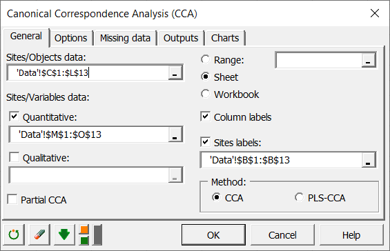
Once you have clicked on the button, the dialog box appears. Select the data that correspond to the sites/species data (here objects are species), and then the sites/variables data (displayed in red color on the Excel sheet).

We also select the sites labels, and make sure the Column labels option is checked so that XLSTAT knows that we included the headers in the selection.

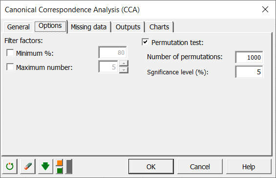
We activate the Options tab, and check the Permutation test option in order to test if the effect of the three variables on the observed frequencies of the insects is significant or not. We decide to run 1000 random permutations.

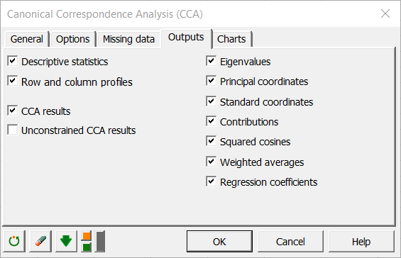
On the two images below, you can see which options have been selected for Outputs and Charts.

After you have clicked on the OK button, the computations start and the results are displayed on a new Excel sheet.

Interpreting the results of a Canonical Correspondence Analysis

The first set of results corresponds to the descriptive statistics of the various variables. The row and column profiles of the contingency table are displayed. The contingency table corresponds here to the frequencies of insects at each site. The "weighted averages" correspond to the means of the variables of the second table, weighted by the marginal sums of the rows of the first table.

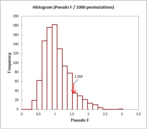
Next we see the results of the permutation test.

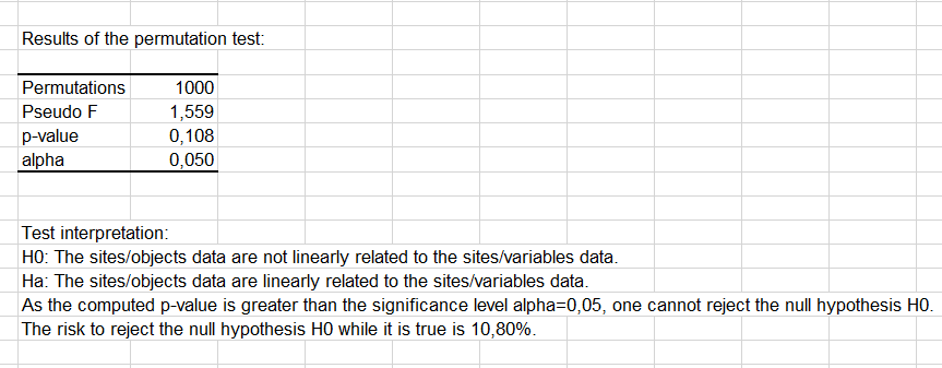
The test concludes that the sites/species data are not linearly related to the sites/variables data with 5% significance level. Looking closer, we see that the p-value is just above the threshold we had chosen (0.05 against 0.089). So the conclusion might not be as obvious. Furthermore, we are interested in checking if this is true for all variables, or if some variables seem to explain the results better than other.

The next table displays how the inertia is spread between the constrained Canonical Correspondence Analysis (the analysis that uses the explanatory variables) and the unconstrained Canonical Correspondence Analysis (the unconstrained Canonical Correspondence Analysis is a Correspondence Analysis of the residuals of the constrained Canonical Correspondence Analysis).

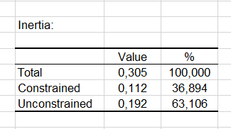
The next table displays how the inertia is spread between the constrained Canonical Correspondence Analysis (the analysis that uses the explanatory variables) and the unconstrained Canonical Correspondence Analysis (the unconstrained Canonical Correspondence Analysis is a Correspondence Analysis of the residuals of the constrained Canonical Correspondence Analysis). We see here that to the constrained Canonical Correspondence Analysis corresponds only 40% of the inertia. So a look at the results of the unconstrained Canonical Correspondence Analysis would make sense, and the relation between the sites and the species should not be analyzed too much in depth here. However, to make the tutorial shorter, we will focus here only on the constrained Canonical Correspondence Analysis results (named simply Canonical Correspondence Analysis results on the report).

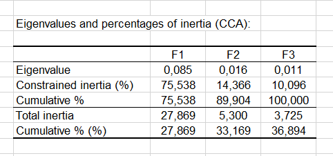
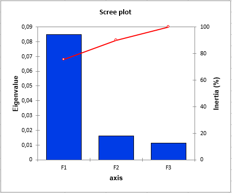
Within the Canonical Correspondence Analysis eigenvector analysis, we see that most of the inertia is carried by the first axis. With the second axis we obtain 92.5% of the inertia. This means that the two-dimensional Canonical Correspondence Analysis map will be enough to analyze the relationships between the sites, the species and the variables.

The Canonical Correspondence Analysis map (see below) allows to simultaneously visualize the objects (here the insect species), the sites, and the variables.

We see on the map that for the species Insect4 and Insect5 the frequency is associated with a high humidity and a low Altitude. Insect7 seems to be more sensitive to the distance to the lake. Insect9 seems to prefer a higher altitude, or more likely a lower humidity.

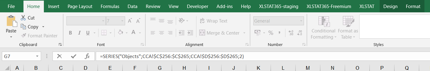
Note: if you want to change the “Objects” to “Species” on the Canonical Correspondence Analysis map, all you need to do is click on one of the points of the corresponding series, and then change "Objects" to "Species" in the Excel formula bar.