Multiple Factor Analysis (MFA) in Excel tutorial
This tutorial will help you set up and interpret a Multiple Factor Analysis (MFA) in Excel using the XLSTAT statistical software.
What is Multiple Factor Analysis?
Multiple Factor Analysis (MFA) is useful to simultaneously analyze several tables of variables and to obtain results, particularly charts, that allow to study the relationship between the observations, the variables, and the tables. Within a table, the variables must be of the same type (quantitative or qualitative), but the tables can be of different types.
The methodology of the Multiple Factor Analysis breaks up into two phases:
-
We successively run for each table a PCA or an MCA according to the type of the variables of the table. One stores the value of the first eigenvalue of each analysis to then weigh the various tables in the second part of the analysis.
-
One carries out a weighted PCA on the columns of all the tables, knowing that the tables of qualitative variables are transformed into a complete disjunctive table, each indicator variable having a weight that is a function of the frequency of the corresponding category. The weighting of the tables makes it possible to prevent that the tables that include more variables do not weigh too much in the analysis.
Dataset for running a Multiple Factor Analysis
The data used in this tutorial have been collected by Asselin C. and Morlat R. from INRA, Angers, France, and used in the following article: [ASSELIN C., PAGES J., and MORLAT R. (1992). Typologie sensorielle du Cabernet Franc et influence du terroir. Utilisation de méthodes statistiques multidimensionnelles. J. Int. Sci. Vigne Vin, 26, 3, 129-154].
The data correspond to the tasting of 21 wines from the Loire region in France by 36 of experts. The dataset comprises 21 observations and 31 dimensions. The 31 dimensions can be grouped into 6 categories:
-
the first 2 qualitative variables are related to the geography (appellation and soil);
-
the next 5 quantitative variables correspond to the olfaction after rest;
-
the next 3 quantitative variables correspond to visual criteria;
-
the next 10 quantitative variables correspond to the olfaction after shaking;
-
the next 9 quantitative variables correspond to the taste;
-
the last 2 quantitative variables correspond to global ratings.
Goal of this Multiple Factor Analysis
The main goal of the study is to understand how the wines relate to each other, and to identify which criteria seem to agree (are redundant?) or disagree. We decide not to use the two qualitative variables and the last two quantitative variables in the first part of the study, but to only use them as supplementary variables at the end of the study: we don't want the analysis to be based on anything else but on objective tasting criteria.
Setting up a Multiple Factor Analysis
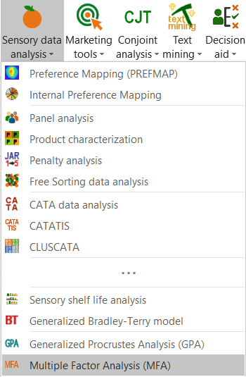
To activate the Multiple Factor Analysis dialog box, start XLSTAT, then select the XLSTAT-Sensory / Multiple Factor Analysis feature in the XLSTAT menu.
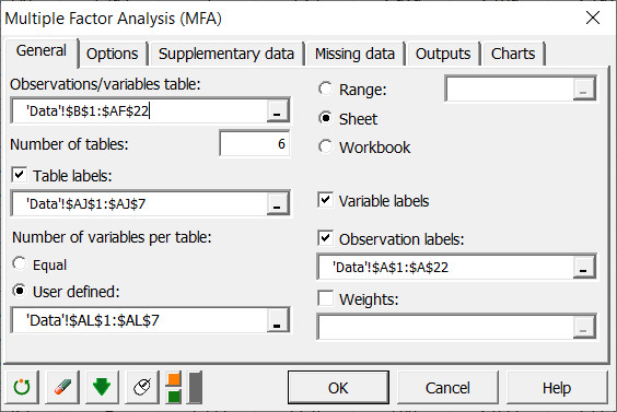
Once you have clicked on the button, the dialog box appears. Select the data that correspond to all the variables of interest. As we saw above, the variables can be grouped into 6 different tables.
So we need to specify that the number of tables is 6. We then select the names we have given to the 6 tables (geog, rest, vis, shake, taste, glob).
Then, we need to define the number of variables within each table. As the number is not the same for all the tables, we need to select a range on the Excel sheet that contains the number of variables within each table.
As the column headers are available in all the selections, we activate the option Variable labels.
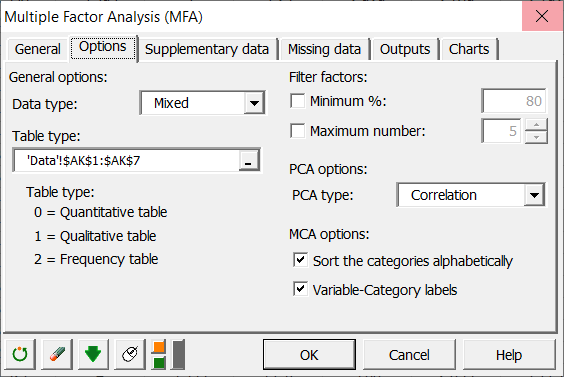
Then click on the options tab to enter additional information.
We have here two types of table: quantitative and qualitative. So we select the Mixed data type, and then we select the column where the types are specified (0 for quantitative, 1 for qualitative).
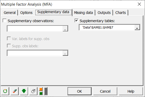
Last, we activate the Supplementary data tab, in order to specify which tables should be taken into account during the initial computations, and which should be only used at the end of the analysis as supplementary tables. Therefore we select the column that defines which tables are active (1) and supplementary (0).
After you have clicked on the OK button, the computations start and the results are displayed on a new Excel sheet.
Interpreting the results of a Multiple Factor Analysis
The first set of results corresponds to the descriptive statistics of the various variables. The statistics that correspond to the variables of the supplementary tables are displayed in blue color.
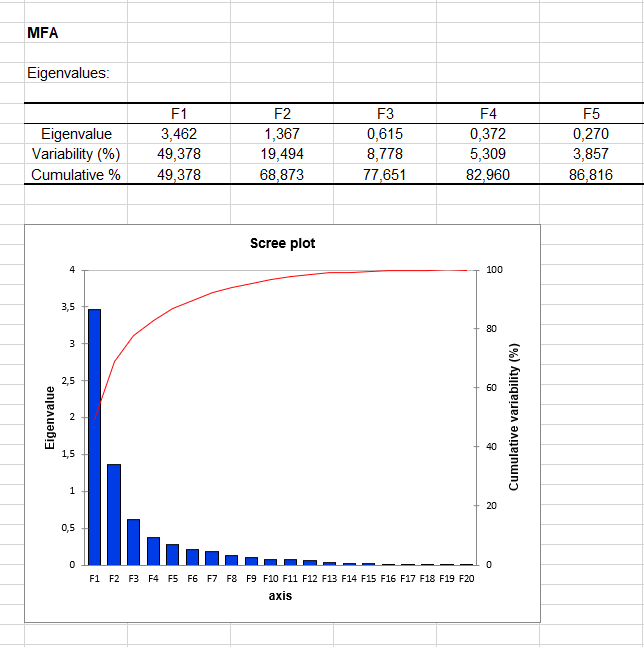
Afterward, separate analyses are run on each table. If the table includes quantitative variables, the analysis that is performed is a PCA (Principal Component Analysis). For tables with qualitative variables, an MCA (Multiple Correspondence Analysis) is performed. So in our case, an MCA is run, followed by 5 PCAs. The results of these preliminary analyses are then used in the final analysis, the second phase of the Multiple Factor Analysis, which is, in fact, a weighted PCA (the weights are set on the columns). The results of the MFA start with the analysis of the eigenvalues of the weighted PCA.
We can see here that with the first two factors we have almost 70% of the variability.
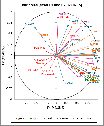
Next, we analyze the correlation map of the variables. This map shows that the two general ratings (typicity and global quality) are highly related to a few variables (Shake3, Taste5 for example), and they are correlated with the first factor. We can also confirm the fact that the vision variables are highly correlated with the first axis. We also see that the various "olfaction after shaking" variables are spread in three of the four quadrants. Last, the second factor is highly correlated with the Rest5 variable.
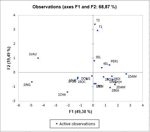
The next chart shows the observations with the centroids of the two qualitative variables. We can see that the T1 and T2 wines are very close, and isolated from the other wines. They are highly related to the second factor, which, as we saw earlier, is highly related to Rest5. The 1DAM wine has the highest coordinate on the first axis. We can also see that the 2DAM wine is in the direction of the two global judgement variables (typicity and global quality). These are the two preferred wines. We can see that the "Ref" SOIL is the soil that is in that same direction. On the opposite, the 1VAU and 2ING wines have the worst ratings.
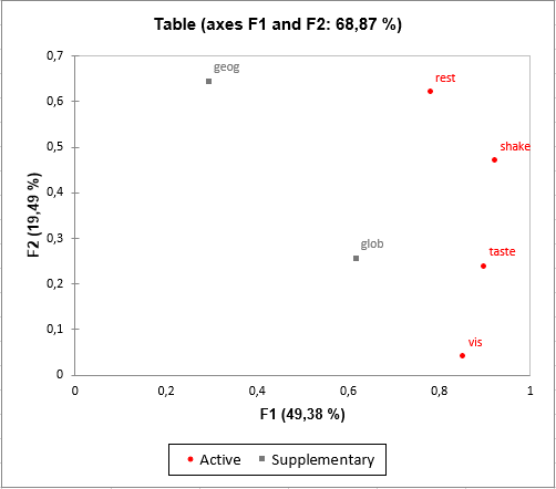
The coordinates of the tables are then displayed and used to create the map of the tables. We can see on the map that the first factor is highly related to the four active tables (high coordinates and high contributions). The second factor is mostly related to the olfaction after rest, and to a lower extent, to the olfaction after shaking.
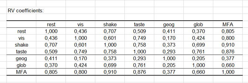
The Lg coefficients of the relationship between the tables allow to measure to what extent the tables are related two by two. The RV coefficients (see below) of the relationship between the tables are another measure derived from the Lg coefficients. The value of the RV coefficients varies between 0 and 1, which make them easier to analyze. We can see here that the two closest tables are the taste and the olfaction after shaking. More surprising, we see that the RV coefficient of the taste and the vision is high.
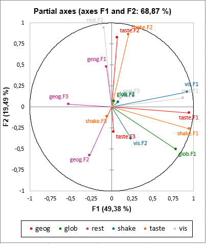
The map of the partial axes allows to see how the factors generated by the separate analyses of the first phase are related to the Multiple Factor Analysis factors. We can see that there is quite a significant relationship between the initial factors and the factors of the MFA. This might however not always be the case.
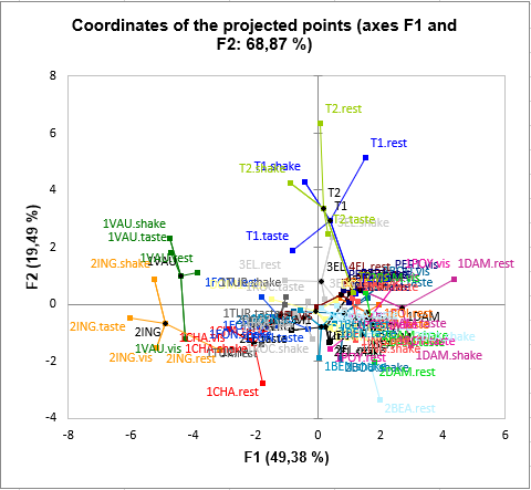
The last chart is based on the previous, but to the observations are added the projected points, and lines are drawn between the observation and the corresponding projected points. The projected points correspond to supplementary observations for which only the information provided by one table is taken into account, the other tables being transformed to 0s. This allows to see how the different tables influence the position of a given point. For example, for the wine T2, we see that the smell at rest tends to make it even more different from the other wines. Looking at other wines, we can see that the smell at rest is often increasing the distance between the wines.
Conclusion
As a conclusion, Multiple Factor Analysis is an interesting and rich method because it makes it possible to analyze complex data sets, and because it provides many graphical results: we can visualize tables (in which variables are grouped), the variables themselves, and the observations. In this particular example, it allowed us to position the wines on a map while being able to quickly interpret their position.
Was this article useful?
- Yes
- No