Building a Bayesian Network in Excel tutorial
This tutorial explains how to build and analyze a Bayesian network (BN) in Excel using the XLSTAT software.
A Bayesian network is a statistical analysis tool based on an acyclic-oriented graph and a probability table. Extremely popular in artificial intelligence, it can be used to represent knowledge and its uncertainties. It is a decision-making tool whose main function is to reveal causal relationships between variables.
Data set to perform a Bayesian network analysis
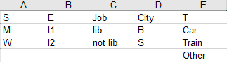
The data come from the “Bayesian Networks with R” book and are used to determine the factors explaining the use of certain transports by a population. We have 6 variables: the age of the individual (Age), the sex (S), the education level (E), the type of job between liberal and non liberal (Prof), the size of the hometown (D) and the type of most used transport (T). The first variable is quantitative while the reste are qualitative. The latter ones have the following modalities:
 The objective of this tutorial is to identify the characteristics of a population regarding the use of means of transport (car, train, etc).
Build and analyze a Bayesian network in XLSTAT
We must first build the Bayesian network which represents the problem, that is to draw the graph and define the probability tables. We choose the one proposed in the book Bayesian Networks with R.
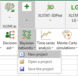
Launch XLSTAT and click on the menu Advanced functions / Bayesian networks / New project as below to open a new project.
 The dialog box Options appears.
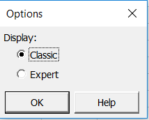 You have the choice to display the Bayesian network feature in a classic mode, which requires the use of a dataset, or in an expert mode, which allows the user to define the data step by step. In this tutorial, we choose the classic mode.
A workbook with 2 sheets opens. The first, called Data, is used to copy/paste the data and the second, called BNGraph, is used to draw the graph.
On the drawing sheet, a toolbar composed of 8 buttons is displayed which serves the different stages of the BN construction and analysis.

A. Draw the graph of the Bayesian network
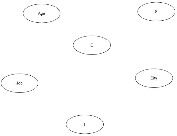
Start by placing the 6 variables using the Node button, the first one of the toolbar. To do this, click the Node button, then go to the drawing sheet where you want to position your node. A window opens aksing to name your node. Repeat this action for each node until you get the following variable layout:
NB for MAC users: for technical restrictions, the node naming window opens only with the second button of the toolbar. To use it you must select before a node with Ctrl + left click.
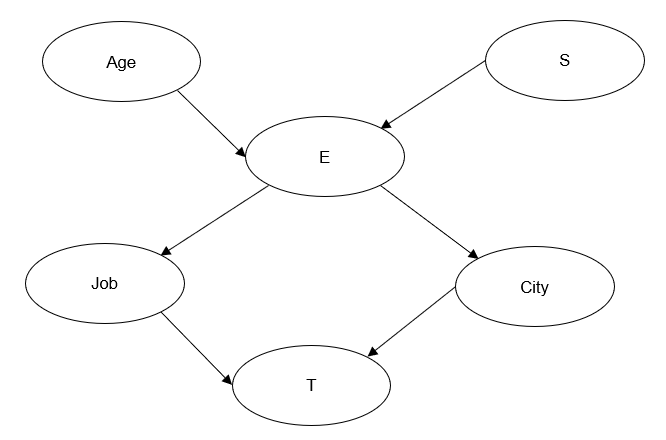
The next step is to draw the causal relationships between the variables using the Arc button, the third one of the toolbar. To do this, select a causal variable, that is a parent node, using the Ctrl key and left click. In the same way, select an effect variable, or child node. As soon as the two nodes are preselected in the correct direction, click on the Arc button. An arrow then appears between the two nodes. In this tutorial the education level, modeled by node E, depends on the age. This relationship is represented by an arrow starting from the node Age and ending to the node E. Create the set of arrows until you get the following graph:
B. Define the probability tables
For all the variables you must define the values for each of modality according to their dependency structure. The node E has two modalities, l1 and l2, and depends on the nodes Age and Sex. It is therefore necessary to define the probabilities of the modality l1, and also l2, knowing the modalities M and W of the sex node and the different age classes of the population. These values are automatically computed by clicking the Data button, the fifth one of the toolbar.
A dialog box appears with two tabs.
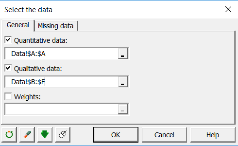 In the General tab, select the data ranges from the Data sheet. Here, columns B to F are selected in the Qualitative field and column A in the quantitative field.
In the Missing Data tab, select the first option to stop computations when missing data is present.
Then click on the OK button to launch the computations. A new Excel sheet appears named Probability tables in which we can find the probability distributions of each variable as well as descriptive statistics of your data.
For example, we see that the variable Age has 3 modalities with the last onew being the most frequent.
Once all the probability tables are completed, the Bayesian network is ready to be analyzed.
C. Launch the Bayesian network analysis
Click the Run Analysis button under tables in the Probability table sheet or directly on the seventh bouton of the toolbar.
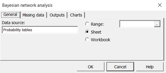
A dialog box appears with four tabs. In the General tab check the name of the pre-selected data source containing the probability tables.
 In the Missing Data, Outputs and Graphics tabs, keep the options checked by default.
Click the OK button to start the computations. The results are displayed in a new sheet called Bayesian Network Analysis.
Interpreting Bayesian network analysis results
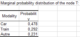
The results are tables and graphs presenting the marginal probability distributions of each node, the join probability distributions of each clique, and the conditional probability distributions.
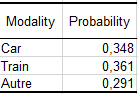
The use of the car is higher compared to the the other means of transport.
 The marginal probabilities of the other variables suggest that half of the population is female, that the number of individuals qualified as l2 is more important than l1 (69% versus 31% respectively) but with almost the same proportion of liberal and non liberal professions (47.9% versus 52.1% respectively). Finally more people live in big cities than small ones (61.9% versus 38.1% respectively).
Conditional probabilities give us more accurate information. For example, we know that a person of a liberal profession uses the car more often than a person of a non liberal profession when we compare the first and fourth lines of the following table:
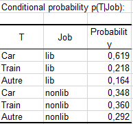 Moreove, the proportion of lib individuals with l2 education level is slightly above the mean compared to the proportion of lib individuals with l1 education level when looking at the first and fourth lines of this table:
Going further with Bayesian networks
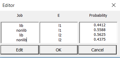
It is possible to modify one or several probability values using the Editor button and relaunch the NB to obtain new results.
To do this, select a node of the BNGraph sheet with Ctrl + left click and click the button. A window then opens, like this one for the node Job:
 We change the probabilities to 0 and 1, respectively, for the two modalities of Node E, to keep the sum equal to 1. To do this, select the first value and click Edit. Enter the new value and click OK. Similarly, modify the other three values to obtain this new probability table:
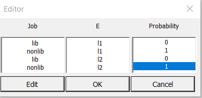 To have these new values reflected in the probability tables sheet, click OK again. You can then run a new analysis taking into account the new marginal probability values of the node.
 For this new Bayesian network, the use of the train is now preferred in a slightly higher proportion than the use of the car.
Was this article useful?
- Yes
- No