Choosing an appropriate time series analysis method

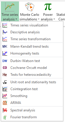
This guide describes time series analysis tools and will help you figure out which method best fits your needs. All the methods mentioned below can be found under the Time Series Analysis menu in XLSTAT, except for linear regression, which is found under the Modeling data menu.

What is a Time Series?

A time series is a sequence of data points aligned in a time order. Data are usually equally spaced. Time series appear in a wide variety of fields. In econometrics and finance, time series include exchange rates, stock prices as well as many other types of variables followed through time. In meteorology, monthly rainfall or temperature measurements taken over several years are considered as time series.

First thing to do: visualize the time series

It is recommended to first visualize the time series to detect potential outliers or visually uncover trends, seasonal behaviors or other common patterns that will be discussed further below. Time series visualization is the first feature that appears under the Time Series analysis menu in XLSTAT. This feature provides the option of displaying several times series simultaneously.

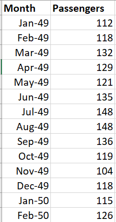
Below is an example of monthly international passenger data (in thousands) from at the San Francisco airport from January 1949 until December 1960. Data are taken from [Box, G. E. P., Jenkins, G. M. and Reinsel, G. C. (1976) Time Series Analysis, Forecasting and Control. Third Edition. Holden-Day. Series G].

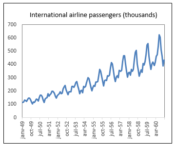
The number of passengers time series is displayed as a line plot in the chart below:

Next steps depend on the question

Several questions can be asked out of time series data:

• After removing the noise, what are the global features in a time series, in terms of trend, seasonal patterns and variance?
• How to relate time-dependent variables? For instance, can we explain household consumption by income based on historical monthly data?
• How to forecast future values of a time series?
• How to measure cycles in a time series?

Each of these questions will be addressed in a different section hereafter.

Investigating trends, variance, and seasonal patterns

What are the main features of the time series displayed in the chart above?

a. Trend and mean of a time series

One of the most interesting things to note on a time series is its global trend, regardless of noisy variations around it. The idea is to study how the mean of the time series changes through time. It seems obvious that there is a positive trend across time in the passengers time series. The number of passengers increased from 1949 to 1960.

The Smoothing feature using the Moving Average option helps uncovering the shape of the global trend while excluding noise.

Mann-Kendall’s nonparametric test can be used to investigate the significance of a globally increasing or decreasing trend. Sen’s slope measures the strength and direction of the trend. Mann-Kendall’s test is significant on the passengers’ time series.

Homogeneity tests, including Pettitt’s, SNHT, Buishand’s and Von Neumann’s, help checking whether there is an abrupt change in the mean of the time series somewhere in time. They all reveal the specific time point where the change occurs, except for Von Neumann’s test.

b. Variance of a time series

Time series may exhibit changing variance across time. This is the case of the Passengers time series, where variance increases through the years. This is reflected by the increasing width of the time series through time.

c. Seasonality in a time series

Lastly, a similar pattern seems to repeat itself year after year: passengers number peaks during the summer months. There is a clear pattern of seasonality.

d. Decomposing a time series into trend and seasonal components

Using the Time Series Transformation feature, it is possible to split the time series into several components including trend, seasonal as well as remaining random noise. There are two possible options:

• Additive decomposition: the original time series can be reconstructed by adding together the three components.
• Multiplicative decomposition: the original time series can be reconstructed by multiplying the three components together. This option is more appropriate when the variance of the time series is changing.

The chart below shows a multiplicative decomposition of the Passengers time series.

How to relate time-dependent variables?

a. Using standard linear regression models on time series: the importance of stationarity

Regression models help explaining one dependent variable by a series of independent variables. For instance, one can be interested by finding out which variables including stock prices or management actions best explain the turnover of a business.

When data used in regression corresponds to historical data such as monthly turnover and stock prices during several years, results may be misleading because of spurious correlations. Imagine a software company seeking to model its revenues according to other factors, based on monthly data during the past year. In a case where there has been an increase of the revenues month after month, revenue is likely to exhibit strong relationships with any random variable showing a month-to-month increase in the past year, even variables that have nothing to do with software sales, such as rainfall or crime rates or admissions at a specific university in a remote country... Variables with trends over time should thus be transformed.

In addition to the absence of a trend, other properties in time series should also be checked prior to using them in regression analysis, such as constant variance and absence of seasonal or more generally, cyclic behaviors. In addition, the time series should not correspond to a random walk. A time series having all these properties is called stationary. Stationarity can be tested using unit-root and stationarity tests, including Augmented Dickey-Fuller, Phillips-Perron as well as KPSS. Here are a few time series transforms which help getting them closer to stationarity when needed for regression analysis.

b. Achieving stationarity: removing trends and seasonality with differencing

One way to remove time trend components in both the dependent or the independent variables is differencing the trended series. Differencing a series means computing time-step change of data values. In the case of the monthly revenues’ variable, that would correspond to using the month-to-month change in revenues. Differencing can also be done at the seasonal scale to remove any seasonal pattern, as seasonality may also lead to spurious correlations.

In a way, this procedure helps removing possible serial autocorrelation among model residuals. Serial autocorrelation can be specifically tested using Durbin-Watson’s test. Nevertheless, in the case of serially autocorrelated data, one may also use Cochrane-Orcutt’s model on the original data. This is a regression model incorporating a correction of serial autocorrelation.

c. Achieving stationarity: reaching constant variance

In many modeling and forecasting procedures such as linear regression or ARIMA models, it is advised to work on time series with constant variance. To check whether a time series has constant variance, one can use heterogeneity tests such as Breusch-Pagan or White tests. These tests are also often performed on the residuals of a regression model to test for homoscedasticity. Some time series transformations such as the logarithm or the Box-Cox transform help making the variance more homogeneous. The Box-Cox transform can be found in the Time Series Transformation feature.

d. Checking if there could be a link between several time series on the long run

Cointegration tests can be used to check whether several time series share an underlying stochastic trend, leading them to an equilibrium on the long run. They are often used in finance to investigate the link between exchange rates.

How to forecast future values of a time series?

Forecasting future values of a specific variable is a main concern in time series analysis. For example, food retailers forecast the number of items likely to be sold in the coming month to adapt stocks in their warehouses. Weather forecasters predict temperature and rainfall amounts during the following days. Many forecasting methods exist. Main available methods in XLSTAT are compared below. They all provide confidence intervals measuring how uncertain the forecast is.

a. Forecasting using linear regression

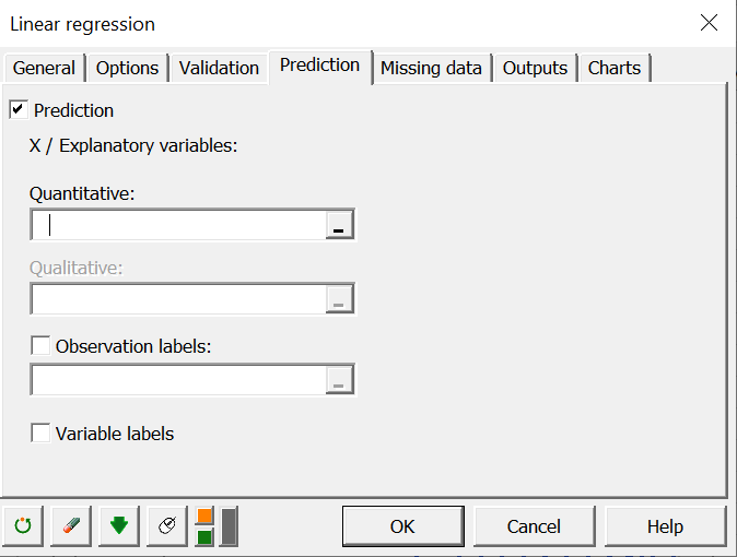
Once a linear regression equation is set, it can be used to forecast values of the dependent variable according to new values of the independent variables, which can be real or inspired by a scenario. For instance, revenues can be forecast using hypothetical scenarios involving specific values of stock prices or marketing investments. In order to obtain regression forecasts in XLSTAT, use the Prediction tab in the linear regression dialog box.

b. Forecasting using exponential smoothing

Exponential smoothing methods help forecasting a time series on its own. They do not incorporate the possibility to include the information from independent variables. They are based on the idea that most recent values should be given a maximum weight in determining the forecasts. Several methods exist and they can all be found in the XLSTAT smoothing feature.

• Simple Exponential Smoothing: all forecasts are the same value, which is a weighted average of past data, with weights decaying toward the past.
• Double Exponential Smoothing: adds a linear trend to the forecast.
• Holt-Winters linear smoothing: similar to double exponential smoothing, but with more flexibility as it involves an additional parameter.
• Holt-Winters seasonal additive: considers a seasonal component.
• Holt-Winters seasonal multiplicative: considers seasonality as well as changing variance.

c. Forecasting using ARIMA

ARIMA models are a family of statistical methods allowing to model and forecast a time series based on its own past values while optionally incorporating the information of independent variables. ARIMA includes the following components:

• AR (AutoRegressive): a data point at time t is forecast using regression on series at past lags (t-1, t-2…).
• MA (Moving Average): a data point at time t is forecast based on errors of past forecasts.

ARIMA allows for automatic differencing. This is what the I (Integrated) in ARIMA stands for. Seasonal differencing can also be considered.

ARIMA involves several parameters to tune, such as the orders of AR, MA and differencing components, in addition to parameters linked to seasonality. One way to choose the optimal values for the parameters is to perform automatic selection based on optimizing AICc or SBC. Advanced users may also use the Autocorrelation functions (ACF) and the Partial Autocorrelation function (PACF) to choose an appropriate set of parameter values. These functions can be obtained using the Time Series Descriptive Analysis feature.

How to measure cycles in a time series?

Spectral Analysis helps measuring cycle periods in a time series. In other words, it allows estimating the frequency content of the series. XLSTAT also provides a Fourier feature that allows for Fourier and Inverse Fourier transforms with several improvements over the standard Excel Fourier Transform function.