Bradley-Terry model in Excel tutorial

This tutorial will help you set up and interpret a generalized Bradley-Terry model in Excel using the XLSTAT statistical software.

Dataset for running a Bradley-Terry model for pairwise comparisons

The data correspond to those used in the book Agresti [Agresti, A. (1990). Categorical Data Analysis. Wiley]. These are the results of baseball games of the American League of the year 1987.

The goal is to fit a Bradley-Terry model by taking home-field advantage into account.

Data format for a Bradley-Terry model

The classical data format for a Bradley-Terry model is the following:

Each pair of teams is compared and the number of wins for each team are counted in the two columns following. In ties are taken into account, a third column has to be added. If homefield advantage are used, the team 1 is considered to be at home.

Goal of a Bradley-Terry model for pairwise comparisons

In this tutorial, we apply a Bradley-Terry model in order to model the probability of winning or losing in the baseball league. The results of the plays are entered in the analysis and a model is obtained with probability of winning or losing for each team. It enables to take into account the home field advantage and the ties.

Setting up a Bradley-Terry model with home-field advantage

After opening XLSTAT, select the Sensory data analysis / Generalized Bradley-Terry model feature:

Once you've clicked on the button, the dialog box appears.

The format of the dataset is such that you have Pairs/Variable table. The dataset is composed by two tables. The first one is the meeting table and the second table corresponds to the results: the first column is the number of wins and the other one the number of losses. The option Two-way table can be used when data are presented in a contingency table.

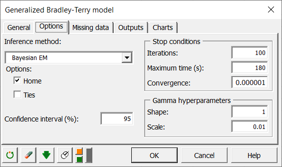
In the Options tab**,** three approaches are proposed to infer model parameters with some option (Home, Ties, stop conditions and Gamma hyperparameters). The confidence interval level can also be modified. Here, we choose the Bayesian EM algorithm with Home option and we have left all the other options to their default values.

The computations begin once you have clicked on OK. The results will then be displayed in a new sheet.

Interpreting the results of a Bradley-Terry analysis

The first results displayed are the statistics for the various teams.

Hereafter are the results for the available dataset. We can notice that the value of Home parameter is 1.76. It means that being at home improve the probability of winning.

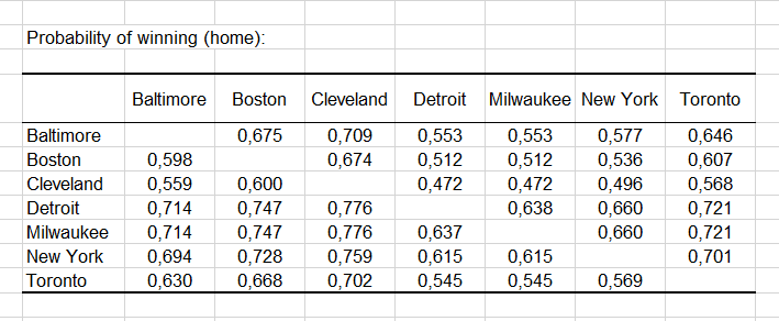
The probabilities of winning are then displayed, followed by a graph that allows you to quickly compare those probabilities. For example, knowing that the Detroit team is at home, the probability that they will beat the Cleveland team is 0.776. We can see from the graph that this is the highest probability for all pairs of teams combined.

The generalized Bradley Terry model can be applied in other cases. For example, to compare products in a sensory test.