Multiple Correspondence Analysis (MCA) in Excel

This tutorial will help you set up and interpret a Multiple Correspondence Analysis in Excel using the XLSTAT software.
Not sure if this is the right multivariate data analysis tool you need? Refer to this guide.

Dataset to run a Multiple Correspondence Analysis

The data correspond to a survey conducted by a car dealer where 28 customers were asked five questions, one week after they had picked up their car after a mechanical repair. The questions were:

• Are you globally satisfied with the service? (Yes/No)

• Do you consider the problem is solved? (Yes/No/Don't know)

• How good was the welcome? (1 to 5)

• Is the quality/price ratio satisfactory? (Yes/No)

• Will you use our services again? (Yes/No/Don't know)

Goal of this tutorial

By running a Multiple Correspondence Analysis (MCA), we want to identify the relationships between the various possible answer to the questions.

Setting up a Multiple Correspondence Analysis with XLSTAT

• After opening XLSTAT, select the XLSTAT / Analyzing data / Multiple Correspondence Analysis command.

• Once you've clicked on the button, the Multiple Correspondence Analysis dialog box appears.

• The format of the data is here Observations/Variables. Select columns B-E in this field.

• The Observations labels are selected in the corresponding field, and the Variable labels option is left activated as the first row of the table contains the name of the variables.
  

• In the Options tab the 1/p option is our filtering choice: the detailed results corresponding to factors which eigenvalue is less than 1/p (where p is the number of active qualitative variables), will not be displayed.

• In the Supplementary data tab: the Come back variable is used as a supplementary variable because we don't want it to influence the computations; however, we want to know how the categories of this variable are positioned on the correspondence map.

• In the Outputs tab. Select the Disjunctive table and Eigenvalues.

• The computations begin once you have clicked on OK. The results will then be displayed.

Interpreting the results of a Multiple Correspondence Analysis

The first results displayed are the tables used for the computations (full disjunctive table, Burt's table).
The total inertia is equal to 2. It depends only on the number of variables and categories and not on the linkage between the variables. Therefore, there is no possible statistical interpretation.

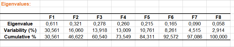
The next table shows the eight non-null eigenvalues and the corresponding % of inertia. However, unlike with CA (correspondence analysis performed on only 2 variables), the % of inertia are here pessimistic estimates of the quality of the representation, the latter being for the user "how close is the representation to the reality".

Then, a table displays the coordinates of the categories in the factors space. The results that correspond to the supplementary variable are displayed in blue color.
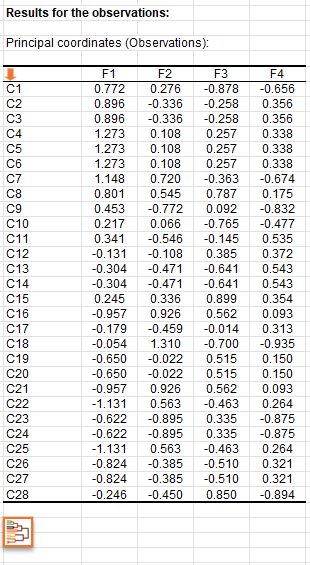
The coordinates of the observations are displayed further down.
The contributions, the test values and the squared cosines help in the interpretation of the results. Before interpreting that two categories are close on the map, one should check that their contribution to the axes of the map, or that their squared cosines are high.
The three following charts respectively correspond to the map of categories, the map of observations and the biplot containing both coordinates of observations and categories on the first two axes.

From these charts, we may suggest that a customer will come back only if he is satisfied with the intervention, the welcome and the price. We also notice that there seems to be a link between the fact that the repair was not satisfactory and the fact that the welcome was bad. This should be investigated further: has the customer described the problem not precisely enough because he had been badly welcome or has the person called back to mention that the problem was still there and has been badly welcome by the representative?

Going further

Running an Agglomerative Hierarchical Clustering (AHC) after a MCA

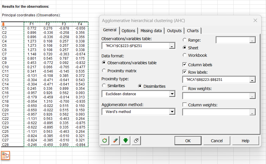
You can launch an AHC by clicking on the button below the table of principal coordinates. An orange arrow allows you to go directly to the end of the table if it contains many variables.

By clicking on this button, the AHC dialog box is then automatically configured and you just have to click on the OK button to launch the analysis.

Click here to see how to interpret the results of the AHC analysis.

Watch our video on MCA analysis

The following video shows you how to run this tutorial.