Multidimensional Scaling (MDS) in Excel tutorial
This tutorial will help you set up and interpret a Multidimensional Scaling (MDS) analysis in Excel using the XLSTAT software.
Not sure if this is the right multivariate data analysis tool you need? Check out this guide.
What is Multidimensional Scaling?
Multidimensional Scaling (MDS) is a data analysis method which is widely used in marketing and psychometrics.
The aim of the methods is to build a mapping of a series of individuals from a proximity matrix (similarities or dissimilarities) between these individuals. In the ideal case where we have a matrix giving the distances between some points on a surface (for example the cities of a country), the Multidimensional Scaling allows rebuilding the exact map of the points (within about a symmetry and/or rotation).
To build an optimal representation, the Multidimensional Scaling algorithm minimizes a criterion called "Stress". The closer the stress is to zero, the better the representation.
Dataset for Multidimensional Scaling
The data correspond to a survey performed over 10 testers which have been asked to rate (the score ranges from 1 to 5) five chocolate bars, where only the product P1 is already available on the market.

Goal of this Multidimensional Scaling analysis
Our aim is to show how the products position themselves on a map, given the opinion of the testers.
Setting up a Multidimensional Scaling analysis
Creating a proximity matrix
A proximity matrix is needed to perform a Multidimensional Scaling analysis, but here we have a individuals x products table. Therefore, we need first to compute the dissimilarities between products, which can be done by using the Similarity /Dissimilarity matrices tool of XLSTAT.
Once XLSTAT is activated, click on the Describing data menu and select Similarity/Dissimilarity matrices (see below).

The dialog box appears. You can then select the data on the Excel sheet and choose the appropriate options as shown below. We decide to display the proximity matrix just below the original data, on the same sheet.

The proximity matrix is generated by default and does not require to be specified as a specific output. The computations begin once you have clicked on OK.
You then obtain the matrix of the euclidean distances between the products, which will be the base for the Multidimensional Scaling analysis.

Setting up the Multidimensional Scaling dialog box
Then click on the Analyzing data menu and select Multidimensional Scaling command (see below).

The Multidimensional Scaling dialog box appears.
You can then select the distances' matrix on the Excel sheet and choose the appropriate options as shown below.
The absolute model has been chosen; this model makes that the distances in the final representation are as close as possible to the initial Euclidean distances.
Other options can give similar results, but a scale effect might be introduced, which we want to remove here.
We ask that the analysis is being performed from 4 to 2 dimensions to evaluate the distortion associated to the decrease in dimensions.

Note: unless you give the algorithm a starting point in the Options tab, the starting points are randomly chosen. Therefore, it is likely that the results you will obtain are slightly different from the one you see on this page. However, it shouldn't alter the interpretation. To be sure that the algorithm finds a true optimum (in terms of stress) you can increase the number of repetitions, the maximum number of iterations, and the accuracy.

The computations begin once you have clicked on OK. After you have accepted to plot the map on the first two dimensions by clicking Done, the results are displayed on the Multidimensional Scaling sheet of the Excel workbook.
Interpreting the results of Multidimensional Scaling
The first table shows the evolution of the stress when the number of dimensions increases. We notice a strong rupture between the 2-dimensional and 3-dimensional representations and a stability between 3 and 4 (it is mathematically normal that a 4D representation for 5 points is perfect).

A map is created on the Dim1 x Dim2 plan, for the 2-dimensional configuration.

It is also possible to build maps for some other couples of axes for the 3 or 4D configurations. However, it is not recommended to view in two dimensions the map for a configuration which has been built for more dimensions, as there might be a projection effect that makes false any interpretation. The 2D map should be used only for the 2 dimensions configuration. To view on a 2D map the 4D configuration, one should first do a PCA on the coordinates.
In order to obtain an even better quality of representation, we use XLSTAT-3DPlot to plot the data in three dimensions.
To do that, we need to select the data:

And to click on the XLSTAT-3DPlot button in the Visualizing data menu:

The result we obtain is as follows:
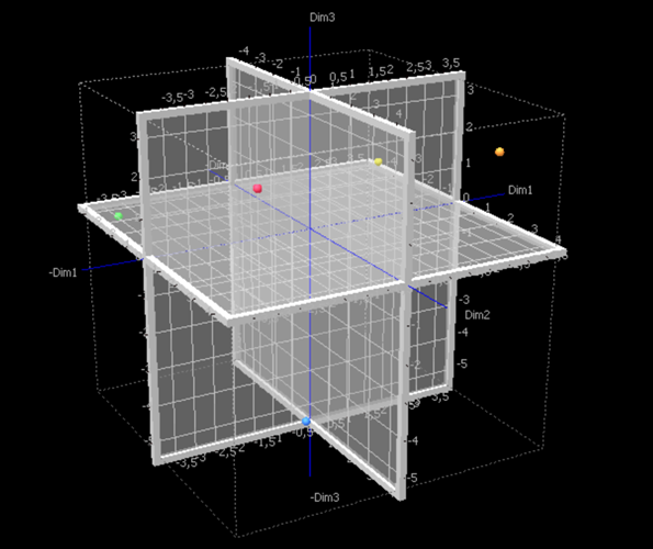
It is possible to see that the testers have collectively well distinguished the products among each other. We know that the product P2 contains more chocolate than P4, which is the one that contains the less chocolate: on the 3D chart, we can see that they are diametrically opposed. By looking at the initial data set, we can see that the testers have significantly preferred the product P2. We can also see that, although they have similar average scores, the products P3 and P5 are not close in the representation space: the testers' opinions are sometimes opposed. That can be explained by the fact that some peanuts have been added to the product P3, which is appreciated by some testers and not by some others.
Conclusion about Multidimensional Scaling
As a conclusion, the Multidimensional Scaling method allows to map the products that have been rated by the testers. It allows a much richer interpretation than simple statistics would.
Note: there is no rigorous statistical method to evaluate the quality and the reliability of a representation produced by a Multidimensional Scaling analysis. However, by looking at the Shepard diagram, one can have a global idea of the quality of the representation. The Shepard diagram corresponds to a scatter plot, where the abscissas are the observed dissimilarities, and the ordinates, the distance on the configuration generated by the Multidimensional Scaling. The disparities are also displayed. The more the points are spread, the less the Multidimensional Scaling map is reliable. If the ranking of the abscissa is respected on the ordinates, then the chart is reliable. If the points are on the same line, then the quality is perfect.

The chart on the left corresponds, for the data used in this example, to the representation in a 4D space. The chart on the right corresponds to the representation in the 2D space. We notice a strong difference of the spread of the points between the two charts.
Note: for an absolute model the disparities are equal to the dissimilarities, which is why they are confounded with the line for the 2D space, and hidden behind the distances on the 4D Sheppard diagram.
The following video addresses Multidimensional Scaling with an illustration in XLSTAT.
Was this article useful?
- Yes
- No