Price Sensitivity Meter in Excel

This tutorial shows how to perform the Price Sensitivity Meter method in Excel using the XLSTAT statistical software.

Dataset to analyze the data with Price Sensitivity Meter

The example below corresponds to a survey on the price of the laptops of middle of the range. Although the number of data and the granularity of the prices is low, we use “Price Sensitivity Meter” of Van Westendorp to analyze what would be the acceptable price range for such a laptop and to determine for the interviewed population which would be the optimal price for an optimal number of sales or an optimal revenue.

Set up the Price Sensitivity Meter dialog box

Once XLSTAT is launched, select the Advanced Functions / Marketing Tools / Price Sensitivity Meter menu.

After clicking on the button, the Price Sensitivity Meter dialog box appears.

In the General tab, select the four variables "Too cheap", "Cheap", "Expensive", "Too expensive" in the Price Data field. Since this selection includes the name of the variable, check the option Column labels.

If Check consistence is checked, XLSTAT will check that the prices are in ascending order for each individual. Otherwise, the individual will not be taken into account for the analysis.

Then select the variables "Score-BM" and "Score-CH" in the Purchase Intent data field.

Click on the OK button to start the calculations.

Interpret the results of Price Sensivity Meter

The descriptive statistics allow in particular to identify the values minimum and maximum. The amplitude is calculated on the too cheap price and the too expensive price. We note in particular that for at least a person, the gap is 1200 Euros what is rather important. For this type of price sensitivity analysis, the usual result is a graph presenting a series of curves whose intersections determine critical prices: from the survey data, six cumulative distribution curves (or their opposites) are computed, first for the four types of prices collected (too cheap, cheap, expensive, too expensive), then, by deduction, we calculate the distribution for not cheap and not expensive.

For too cheap and cheap, we take the opposite of the distribution curve. For each of the prices indicated by the panel participants, we calculate what proportion of respondents s indicated a higher price. These curves therefore decrease from 1 to 0 when the price increases. For expensive and too expensive, we take the cumulative distribution curve. Therefore, for each of the prices indicated by the respondents, we calculate what proportion of consumers indicated a lower price. These curves therefore increase from 0 to 1 when the price increases.

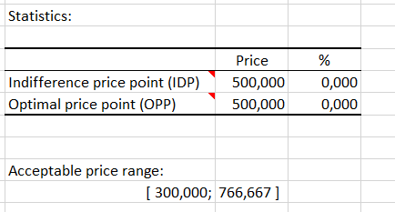The intersection between the cheap and expensive curves is the price for which the same number of panelists consider the product to be expensive or cheap. Even if it is not necessarily strong, there is a disagreement between these two groups of same size of respondents on this price which has been named Indifference Price (IDP). According to Van Westendorp, this price corresponds to the reality of the market. The IDP can be interpreted as the median market price for this type of product or as the price offered by a market leader. This is the right price point for a majority of respondents, a small proportion finding it cheap (probably not expensive enough for the company marketing this product) or expensive (potentially at risk for of a concurrent). Of course, an even smaller respondents will find it too cheap (suspicious quality) or too expensive (inaccessible).

The intersection between the curves of too cheap and too expensive corresponds to the price for which people consider the product to be too expensive or too cheap. This price, which corresponds to totally opposed opinions, concerns few consumers. This price is called the Optimal Pricing Point (OPP), in the sense that as many consumers as possible should be able to buy the product.

In this example IDP and ODP prices are both equal to 500€. The range of acceptable price goes from 300€ to 766€.

The acceptable price range is given by, for the lower bound, the intersection between the too cheap and not cheap curves, and for the upper bound, by the intersection of the too expensive and not cheap curves. Between these two marginal prices, the authors estimate that sales volumes are high. XLSTAT allows its users to take into account the contribution of Newton et al. (1993) who proposed to take into account the purchase intent within the framework of the survey, by asking what is the purchase intent score, for the cheap and expensive prices. These scores can be transformed into probabilities, either automatically or through a conversion table. Once probabilities are available, we can identify which price is likely to generate a maximum volume of sales and which price is likely to generate a maximum revenue. In this example, the scores of intention of purchase from 1 to 5 are automatically translated into probability 0 / 0.1 / 0.3 / 0.5 / 0.7.

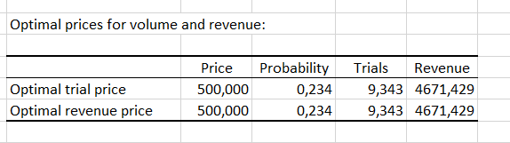The consideration of the intentions of purchase allows to define the price of the product by maximizing the chances that the impact is favorable on the volume or the revenue according to the chosen strategy. In the table above, we see that the price allowing to maximize both criteria is 500€.

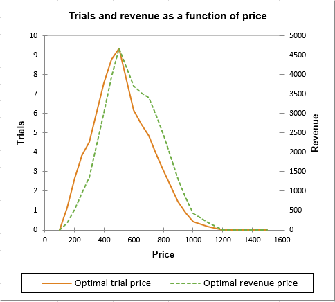The graph above allows to observe the evolution of the volume and the revenue according to the prices. We see that the optimum is clearly equal to 500€. On the basis of the collected data, the method of the Price Sensitivity Meter allows us to pronounce on the optimal price of a mid-range laptop. Naturally, this conclusion totally disregards the competitive situation and the impact of the mark of the laptop.