elasticidad precio de demanda (PED) tutorial en excel

This tutorial shows how to compute and interpret Price elasticity of demand (PED) in Excel using the XLSTAT statistical software.

What is Price elasticity of demand?

Price elasticity of demand (PED or Ed) is an important concept in economics, and obviously a very important metric for any company or organization that sells a commodity for which it has some freedom to change the price. This means that the price must not be fixed by an external organization of by a very strict competitive situation. Setting or adapting the price of a product is something that makes a lot of managers afraid, while it is one of the most strategic decision to make. A well-planned price change can boost profits and create a virtuous dynamic in a company.

The concept was explored in depth by Alfred Marshall in his book “Principle of Economics” first published in 1890 (see Book III, Chapter IV, https://oll.libertyfund.org/titles/marshall-principles-of-economics-8th-ed). Macgregor (1942) wrote an interesting historical review of the contributions on the subject with references to earlier works.

Price elasticities are often used by economists to compare commodities and how consumers react to a single price change. For example, how does a price change on soft drinks compares to a price change on fruits? Our example below corresponds to a case where we compare how different populations react to a price change. Check out our article What is Price elasticity of demand for a more theoretical background.

Dataset to compute Price Elasticity of Demand

The data corresponds to a test that was run at two supermarkets on the price of pineapples. The price was changed for the study between $2.49 and $3.99 by steps of 10 cents. Each price was tested for one week. To avoid a misleading effect of the variation of general traffic, the quantities sold have been corrected considering the total number of people visiting the supermarket each week. The supermarkets are located in two different areas, one with a majority of high-income households and one with mostly low-income households.

Goal of this tutorial

We now want to analyze the results and evaluate the price elasticity. Previous studies on fruits (Durham and Eales, 2008) or comparing low income and high-income households (Jones and Mustiful, 1996) have been used to validate the results.

The tool for price elasticity of demand analysis available in XLSTAT has been used to compute elasticities and display the results. The dialog box allows to directly select prices and demand (here units sold). We choose to compute arc elasticities.

Setting the PED dialog box in XLSTAT

Once XLSTAT is launched, select the Advanced Functions / Marketing Tools / PED menu. The Price Elasticity of Demand dialog appears: In the General tab, select columns A, B and C in the Prices, Demand and Groups fields. Here, we choose to compute the arc elasticities. After clicking OK, a series of tables and charts are displayed.

Interpreting the results of Price Elasticity of Demand

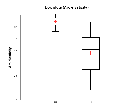
We can see that the price elasticity is most of the time lower for the low-income group than for the high-income group. We can also see that for the low-income group, the higher the price the lower the elasticity, while for the high-income group, the elasticity is always in the same range. To compare the elasticities of the two groups, we then run a t-test with an automatic F-test to verify if the variance is homogeneous across groups. From the outputs of the t-test we extracted the box plots which confirms a significant difference in mean and variance.