What is Price Elasticity of Demand (PED)?

An introduction to Price elasticity of demand

Price elasticity of demand (PED or Ed) is an important concept in economics, and obviously a very important metric for any company or organization that sells a commodity for which it has some freedom to change the price. This means that the price must not be fixed by an external organization of by a very strict competitive situation. Setting or adapting the price of a product is something that makes a lot of managers afraid, while it is one of the most strategic decision to make. A well-planned price change can boost profits and create a virtuous dynamic in a company.

The concept was explored in depth by Alfred Marshall in his book “Principle of Economics” first published in 1890 (see Book III, Chapter IV, https://oll.libertyfund.org/titles/marshall-principles-of-economics-8th-ed). Macgregor (1942) wrote an interesting historical review of the contributions on the subject with references to earlier works.

Price elasticity of demand has been developed to measure how demand relatively varies when prices change. The “relatively” is important in the concept. The idea is that the measure should not depend on the scale or even where on a given scale the measure is done so that it can be compared for different commodities. For example, between a low-cost camera and an expensive camera. Note that economists have also studied the reciprocal problem: if a product becomes abundant on the market, how will it impact prices (think, for example, of how the prices of hand spinners evolved from medium to high and then to low prices, as a function of availability and trendiness).

The term elasticity comes the physical concept. If an object moves, here the price, does the related object, here the demand, reacts at the same pace (elasticity – we say demand is elastic), or is there a slow reaction (inelasticity) or no reaction (perfect inelasticity).

To measure elasticity, you need to measure by how much the demand varies when the price varies from one value to another, or equivalently, by one per cent as some like to do it. So, this would simply be the ratio of the differences. As mentioned above, we want to remove the effect of scale, so that the elasticities for different goods or at different positions on the scale can be compared. As a consequence, we divide the price difference by the initial price and the difference in demand by the initial demand value. In the end, we can write: Ed = [dQ/Q] / [dP/P] Or similarly, Ed=[dQ/dP][P/Q]

The d in mathematics stands for the difference and if Q can be written as a function fd of P (Q=fd(P)), then [dQ/dP] is the derivative of the fd function. However, it is very rare that there is a known function to describe the relationship, and the elasticity must be empirically estimated.

Point Elasticity: If you say prices change from P1 to P2, then you can write the following: Ed(point) = [(Q2-Q1)/Q1] / [(P2-P1)/P1]

When the elasticity is computed this way, it is referred to as Point Elasticity. The problem when you write the equation this way is that Ed depends on whether you change prices from P1 to P2 or from P2 to P1.

Arc Elasticity: To avoid this problem, the Arc Elasticity is often used instead. It is computed at the middle point between P1 and P2: Ed(arc) = [(Q2-Q1)/(Q1+Q2)/2] / [(P2-P1)/(P1+P2)/2] Which simplifies to Ed = [(Q2-Q1)/(Q1+Q2)] / [(P2-P1)/(P1+P2)] or Ed = [(Q2-Q1)(P1+P2)] / [(P2-P1)(Q1+Q2)]

Notes: If revenue is R=PQ, then Ed= R The smaller the difference between prices, the lower the difference between point and arc elasticities.

Some authors take the opposite of Ed to avoid manipulating negative elasticities.

Interpretation:

Mathematically speaking, elasticity is a multiple of the slope coefficient of the line that is tangent to the curve if the quantity is a known function of the price. For the arc elasticity, it is a multiple of the slope coefficient of the line that links (P1,Q1) to (P2,Q2). Though the tangent is often displayed in many documents available online or offline, this is not very helpful.

To facilitate the interpretation, one should remember that elasticity is the ratio of the relative change in prices and of the relative change in quantities. In other words, what’s the value of Ed when the price changes by 1%: by how many % will the quantities vary.

Demand is price elastic if the demand reacts strongly when the price increases from P1 to P2 (P2Q2<P1Q1). It is perfectly elastic if Ed =- ∞. Such an extreme case corresponds to a case where quantities would diminish a lot after a small increase in prices, or reciprocally, if quantities sold would increase a lot when prices decrease a little. Demand is unit elastic with Ed=-1 if demand evolves like prices. As far as turnover is concerned, the drop in the quantity sold is exactly compensated by the rise in prices. Demand is inelastic (or rigid) if the increase of price has a small impact on quantities (-1 < Ed ≤ 0). Demand is perfectly inelastic if Ed=0.

For some specific products (Giffen goods which are essential goods, or Veben goods such as luxury goods). The increase in prices has a significant positive effect on quantities. It is important to note that there is no direct relationship between price elasticity and revenue. When unit elasticity is reached, it corresponds to a case where revenue is stable. In some cases, it might correspond to a maximum or a minimum in revenue.

Though we consider here that the demand is a function of price, which means we should represent the relationship on a chart with demand (or quantities) in ordinates and prices in abscissa, the charts below are displayed the way around, because it is common in economics to study how prices adjust to demand (for example, for low-cost goods that are massively available, or airline fares).

Let’s build a few cases to understand how the curves would look like with different types of elasticities. Imagine a case where quantities sold diminish linearly with the increase in prices with a slope a (Q=aP+b). This means that Ed=a(aP+b)/P. Figure 1 corresponds to a case where a=-1 and b=195. We can see that on the lower part of the price range, the demand is elastic, and it becomes inelastic when prices increase. Figure 1: Elasticity in a case of linear relationship Note: When reading the revenue on the above curve, to know the price at which it is generated, you need to read the price curve for the same demand value and find the corresponding value on the ordinate axis. In figure 1, the maximum revenue (rescaled for convenience) is obtained at a price of 97.5 and corresponds to elasticity of -1. Above this price the demand is inelastic and below it is elastic. Hereunder we display an example with a hyperbolic relationship between demand and prices. The higher the prices, the lower the impact on quantities. Figure 2: Elasticity in a case of hyperbolic relationship

We obtain the maximum revenue when the price is the highest, but after diminishing until the price reaches 90, it increases again when prices continue to diminish. We see here that unit elasticity corresponds to a minimum revenue.

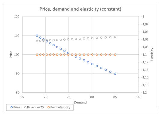
Let’s now build a case where the elasticity is constant. In such a case, we have dQ/dP=eQ/P, where e is the elasticity. The function Q=c(P^e) satisfies the differential equation. We display hereunder an example with e=-1.1. Figure 3: Constant elasticity

In Figure 3 we see that in this specific case, revenue diminishes when price increases. Price elasticities are often used by economists to compare commodities and how consumers react to a single price change. For example, how does a price change on soft drinks compares to a price change on fruits? Check out a practical example provided in the tutorial **Price Elasticity of Demand in Exce**l.

References

Durham C. and Eales J. (2008). Demand Elasticities for Fresh Fruit at the Retail Level. Applied Economics, 40, 1-10. Henderson J. P. (1973). William Whewell's Mathematical Statements of Price Flexibility, Demand Elasticity and the Giffen Paradox. The Manchester School, 41, 329-342 Jones E. and Mustiful B.W. (1996). Purchasing behaviour of higher-and lower-income shoppers: a look at breakfast cereals, Applied Economics, 28(1), 131-137 Macgregor D. H. (1942). Marshall and His Book. Economica. 9(36), 313-324 Marshall, Alfred (1890). Principles of Economics. Macmillan, London.