Generating many distributions in a simulation model by copying
This tutorial will help you set up a simulation model and generate many distributions in Excel using the XLSTAT statistical software.
Simulation models
Simulation models allow to obtain information, such as mean or median or confidence intervals, on variables that do not have an exact value, but for which we either know or assume a distribution. If some “result” variables depend on these “distributed” variables by the way of known or assumed formulae, then the “result” variables will also have a distribution. Sim allows you to define the distributions, and then to obtain, through simulations, an empirical distribution of the input and output variables as well as the corresponding statistics.
Simulation models are used in many areas such as finance and insurance, medicine, oil and gas prospecting, accounting, or sales prediction.
Four elements are involved in the construction of a simulation model:
- Distributions are associated to random variables. XLSTAT gives a choice of more than 30 distributions to describe the uncertainty on the values that a variable can take. For example, you can choose a triangular distribution if you have a quantity for which you know it can vary between two bounds, but with a value that is more likely (a mode). At each iteration of the computation of the simulation model, a random draw is performed for each distribution that has been defined.
- Scenario variables allow to include in the simulation model a quantity that is fixed in the model, except during the tornado analysis where it can vary between two bounds.
- Result variables correspond to outputs of the model. They depend either directly or indirectly, through one or more Excel formulae, on the random variables to which distributions have been associated and, if available, on the scenario variables. The goal of computing the simulation model is to obtain the distribution of the result variables.
- Statistics allow to track a given statistic for a result variable. For example, we might want to monitor the standard deviation of a result variable.
A correct model should comprise at least one distribution and one result variable. Models can contain any number of these four elements. A model can be limited to a single Excel sheet or can use a whole Excel folder.
In this tutorial a simulation model is created that simulates the payment of interest of a in fine loan over 5 years and uses the interest rate of the first year to calculate the net profit value. During this tutorial the copy of distribution cells using the normal Excel copy and paste function is introduced.
Dataset for generating many distributions in a simulation model efficiently
Our simulation model deals with the payments of interest of a in fine loan. The interest are calculated during 5 years. At the end the net profit value at the initial time is calculated using the Excel function NPV and the interest rate of the first year and the payments of interest during the 5 years. The interest rate is support to be equally distributed between 3.5% and 5.5%. The capital of the in fine loan is 10000 Euro.
Starting with a static model using a mean interest rate of 4.5%. The net profit value is calculated to 1975 Euro in that case.

This model can be found in the "Model" sheet.

Generating many distributions in a simulation model efficiently by copying
In the following we use relative references to copy the distributions correctly. Please verify in the Sim Options, that the Relative reference option was activated before creating the distribution variables. This allows that the copy/paste actions change the reference automatically.
Creating the first distribution
Select the first distribution variable in B6, the "interest rate" for 2008, to make it the active cell.
Once XLSTAT is activated, select the XLSTAT / Sim / Define a distribution command, or click on the corresponding button of the Sim toolbar (see below).

The appears. Choose the Excel cell with the name “2008” as name. This will be integrated as a relative reference (A1 format) in the formula.
Choose a uniform distribution with a = 0.035 and b = 0.055.

Once you have clicked on OK, the corresponding function call to XLSTAT_SimDist is inserted into the active cell.
Creating distribution by copying
It is possible to enter the other four distributions using copy and paste of the cell that we have generated into the four cells at the right of this first cell. You have as well the possibility, as with any Excel formula, to select the cell B6 that you have just generated, go with the mouse over the lower left corner where the cursor is displayed as a black cross, press and hold the left mouse button and move the mouse up to the F6 cell. This way you have defined the 5 cells as well. The name of the distributions will be “2008, …, 2012”.
![]()
Choose the result cell B9 that contains the formula = NPV(B6,B7,C7,D7,E7,F7) as active cell. Now the result variable will be defined. Select the XLSTAT / Sim / Define a result command, or click on the corresponding button of the Sim toolbar.
The define result dialog box will appear. Then select the data on the Excel sheet. Choose the Excel cell with the name “NPV” as name in it.
Once you have clicked on OK, the corresponding function call of XLSTAT_SimRes is inserted into the active cell.
This can be found in the Excel sheet Model.
Running the simulation
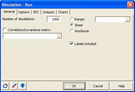
To start the simulation run, select the XLSTAT / Sim / Simulation - Run command, or click on the corresponding button of the Sim.
The simulation - run dialog box will appear. Set the number of simulations to 1000.
In the Options tab, enter the parameters of the tornado and spider analysis. Select the standard cell value as default value. Choose 10 data points in the interval from -10% up to +10% of the value deviation:

The computations begin once you have clicked on OK.
Interpreting the results of the simulation
The first result is a summary of the elements included in the model. Details on the distribution variables and on the result variable are displayed.

The following tables dsiplay descriptive statistics, histograms and quantiles for each distribution variable.

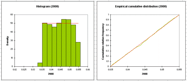
The following tables show details for the result variables (descriptive statistics, histograms and quantiles). Then, results of the sensitivity analysis are displayed. These results depend on the iterations of the simulations.

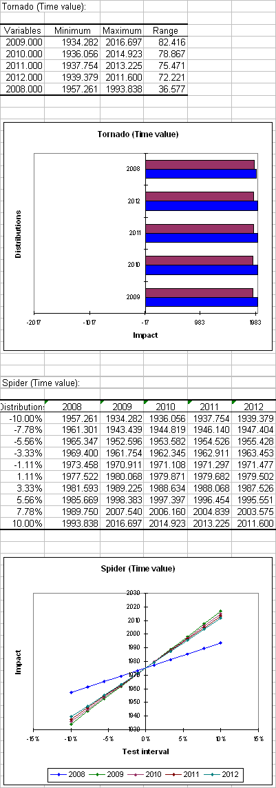
The next section contains the tornado analysis. Tornado and spider analyses are not based on the iterations of the simulation but on a point by point analysis of all the input variables (random variables with distributions and scenario variables).
During the tornado analysis, for each result variable, each input random variable and each scenario variable are studied one by one. We make their value vary between two bounds and record the value of the result variable in order to know how each random and scenario variable impacts the result variables. For a random variable, the values explored can either be around the median or around the default cell value, with bounds defined by percentiles or deviation. For a scenario variable, the analysis is performed between two bounds specified when defining the variables. The number of points is an option that can be modified by the user before running the simulation model.
The spider analysis does not only display the maximum and minimum change of the result variable, but also the value of the result variable for each data point of the random and scenario variables. This is useful to check if the dependence between distribution variables and result variables is monotonous or not.
In the first table the minimal and maximal change and the corresponding range are displayed for each distribution variable. In this case all interest rates are more or less the same. In the spider analysis in the next section we see that the interest rate of the first year has less impact than the other interest rates, because in the formula of NPV the interest rate of the first year is used as well and therefore variations of this interest rate to not have much influence on the NPV.
Was this article useful?
- Yes
- No