Run a simulation model with correlations between distributions and compute SPC (process capability) indicators
This tutorial will help you set up and run a simulation model with correlations between distributions and compute SPC process capability indices in Excel using XLSTAT.
What is a simulation model
Simulation models allow to obtain information, such as mean or median or confidence intervals, on variables that do not have an exact value, but for which we either know or assume a distribution. If some “result” variables depend on these “distributed” variables by the way of known or assumed formulae, then the “result” variables will also have a distribution. Sim allows you to define the distributions, and then to obtain, through simulations, an empirical distribution of the input and output variables as well as the corresponding statistics.
Simulation models are used in many areas such as finance and insurance, medicine, oil and gas prospecting, accounting, or sales prediction.
Four elements are involved in the construction of a simulation model:
-
Distributions are associated to random variables. XLSTAT gives a choice of more than 30 distributions to describe the uncertainty on the values that a variable can take. For example, you can choose a triangular distribution if you have a quantity for which you know it can vary between two bounds, but with a value that is more likely (a mode). At each iteration of the computation of the simulation model, a random draw is performed for each distribution that has been defined.
-
Scenario variables allow to include in the simulation model a quantity that is fixed in the model, except during the tornado analysis where it can vary between two bounds.
-
Result variables correspond to outputs of the model. They depend either directly or indirectly, through one or more Excel formulae, on the random variables to which distributions have been associated and, if available, on the scenario variables. The goal of computing the simulation model is to obtain the distribution of the result variables.
-
Statistics allow to track a given statistic for a result variable. For example, we might want to monitor the standard deviation of a result variable.
A correct model should comprise at least one distribution and one result variable. Models can contain any number of these four elements. A model can be limited to a single Excel sheet or can use a whole Excel folder.
Dataset for running a simulation model integrating correlations between distributions
In this tutorial we add to the model of the first tutorial a correlation matrix and an SPC analysis. Our simulation model is based on sales and costs of a shop. The benefit is simply the difference between sales and costs in this simple case. Based on historical data for costs and sales that were analyzed with the tool “distribution fitting” we found out that the costs follow a normal distribution (mu=120, sigma=10) and the sales a normal distribution (mu=80, sigma=20) (see Histograms and distribution fitting tutorial in Excel or more details).
We suppose that the costs and the sales are correlated with a spearman correlation coefficient of 0.8. This is shown in the correlation matrix. The lower triangle is sufficient. It is important that the headers of the rows and columns are the same as the names given to the the distribution variables when they were defined.
Additionally an SPC analysis for the three model variables is carried out. During the planning for the running year we defined upper and lower specification limits and a target value that is identical to the static model.
Note: The SPC analysis is only available, if a valid SPC license is present.

This model can be found in the Model sheet.
Running the simulation model integrating correlations between distributions and computing the SPC indicators
To start the simulation run, select the XLSTAT / Sim / Simulation - Run command, or click the corresponding button of the Sim toolbar.
The Simulation - Run dialog box appears.
Set the number of simulations to 1000. Activate the Correlation/covariance matrix and select the correlation matrix including the row and column headers.

In the Charts - Sensitivity tab, enter the parameters of the tornado and spider analysis. Select the standard cell value as default value. Choose 10 data points in the interval from -10% up to +10% of the value deviation:

In the SPC tab, if a valid SPC license is present, we activate the calculate process capabilities option.
Choose for the selection field LSL the three Excel cells below the cell LSL, because the column label is not necessary. Fill in USL in the same way.
In the field Name select the 3 cells with the names of the model elements for which the SPC analysis should be carried out: "sales", "costs" and "benefit" located to the left of the model elements.
Last, activate the target option to calculate SPC values that need a target value.

The computations begin once you have clicked OK.
Interpreting the results of a simulation model integrating correlations between distributions and SPC indicators
In the model summary the proximity matrix is displayed: 
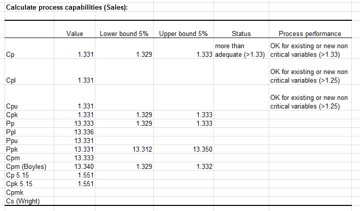
After the following tables that contain the details of the distribution and result variables, additional results of the SPC analysis are displayed:
Finally the correlation matrix of the different distribution and result variables is displayed. We see that the spearman correlation between costs and sales is close to 0.8. If the number of iterations during the simulation was bigger, then this correlation will be even closer to 0.8.

Was this article useful?
- Yes
- No