How to run a simple simulation model with XLSTAT
This tutorial will help you set up and run a simple simulation model in Excel using the XLSTAT statistical software.
Simulation models
Simulation models allow us to obtain information such as mean, median, or confidence intervals about variables that do not have an exact value, but for which we either know or assume a distribution. If some "result" variables depend on these "distributed" variables via known or assumed formulas, then the "result" variables will also have a distribution. The Monte Carlo simulations in XLSTAT allow you to define the distributions and then, through simulations, to obtain an empirical distribution of the input and output variables and the corresponding statistics.
Simulation models are used in many fields, such as finance, insurance, medicine, oil and gas exploration, accounting or sales forecasting.
Dataset for creating and running a simple simulation model
In this tutorial, a very simple simulation model with two distributions and one result is created to explain the basics of simulation modeling. More tutorials with all 4 model elements and options can be found here.
Our simulation model is based on the sales and costs of a business. Profit in this simple case is simply the difference between sales and costs. Based on historical data for costs and sales analyzed with the distribution fitting tool, we found that costs follow a normal distribution (mu=120, sigma=10). Sales also follow a normal distribution (mu=80, sigma=20) - See Fitting a distribution to a sample of data in Excel for more details.
Based on this model, the various model variables are created:
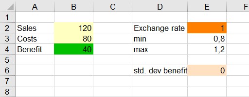
This model can be found on the sheet "Model".
Create a simple simulation model
How to define the distribution variables in XLSTAT?
-
Open XLSTAT.
-
Select cell B2 cell that contains the amount of sales.
-
Click on XLSTAT > Monte-Carlo simulations>Define a distribution. The Define a distribution dialog box appears.
-
Select the Variable Name (sales) in cell A2. Choose a normal distribution with mu=120 and sigma=10. A formula calling the XLSTAT_Sim function is created in cell B2.

-
Start again in the cell below to generate a normal distribution with mu=80 and sigma=20.

How to define the result variable in XLSTAT?
-
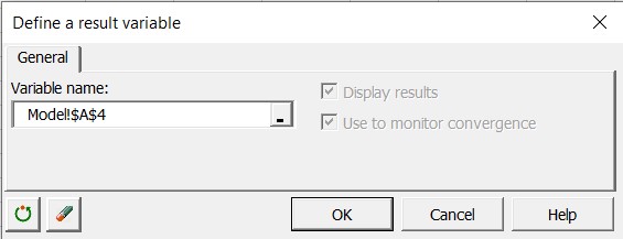
Select the result cell that contains the value 40 as the result of the formula =B2-B3. Note that the result variable must not be constant, but must depend on at least one of the distribution variables defined above.
-
Then click the XLSTAT>Monte Carlo Simulations >Define a result variable command in the XLSTAT menu. The Define a result variable dialog box appears.
-
Select cell A4 as Variable name. The corresponding function call to XLSTAT_SimRes is inserted in cell B4.
Execute a simple simulation model
-
Select the XLSTAT > Monte Carlo Simulations > Run command. The Run dialog box appears. Set the number of simulations to 1000.
-
Set up the Charts > Sensitivity tab as shown in the figure below.

-
Click OK to start the analysis.
Interpret the results of a simple simulation model
The first result is a summary of the simulation model that contains the default values of the cells and the distributions of the variables. It also contains the formula that explains how to compute the result variable.

Several statistical indicators such as mean, median, quartiles, variance, standard deviation and skewness coefficients of the distributions of the two random variables (sales and costs) are shown in the following table.
The following histogram shows the distribution of the Costs variable. A histogram for the variable sales is also shown.
How to interpret the results of the sensitivity analysis?
The same tables and graphs are displayed to examine the result variable after the simulation. This is followed by a sensitivity analysis based on the simulation results. The table below shows the results of this analysis for the outcome variable (Benefit).
We can see, for example, that the evolution of cost contributes almost 80% to the evolution of benefit and that the correlation between these two variables is negative. The higher the cost, the lower the benefit. These results are illustrated in the graph below.
How should the tornado analysis be interpreted?
Tornado analysis is not based on the iterations of the simulation, but on a point-by-point analysis of all input variables (random variables with distributions and scenario variables).
In the tornado analysis, for each result variable, each input random variable, and each scenario variable are examined one by one. We allow their value to vary between two bounds and record the value of the result variable to learn how each random and scenario variable affects the outcome variable. For a random variable, the values examined can be either around the median or around the standard value of the cell, with bounds defined by percentiles or deviation. In the case of a scenario variable, the analysis is performed between two bounds that were specified when the variables were defined.
In both the table and the chart, we see that cost has the strongest influence on benefit. This interpretation results from the width of the tested interval.
Finally, the correlation matrix of the distributions and outcome variables is displayed. We see that cost and revenue are not correlated. But, of course, benefits are correlated with sales and costs.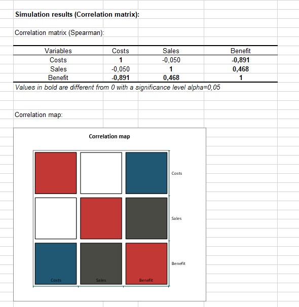
Was this article useful?
- Yes
- No