Simple linear regression in Excel tutorial

This tutorial will help you set up and interpret a simple linear regression in Excel using the XLSTAT software. Simple linear regression is based on Ordinary Least Squares (OLS).

Not sure this is the modeling feature you are looking for? Check out this guide.

What is simple linear regression?

Simple linear regression enables you to predict a variable depending on another variable, on the basis of a linear relationship inferred by a supervised learning algorithm.
If you are trying to predict a variable depending on several others, do not hesitate to read our tutorial on Multiple Linear Regression.

How to run simple linear regression in XLSTAT?

Dataset for running a linear regression

The data have been obtained in Lewis T. and Taylor L.R. (1967). Introduction to Experimental Ecology, New York: Academic Press, Inc.. They concern 237 children, described by their gender, age in months, height in inches (1 inch = 2.54 cm), and weight in pounds (1 pound = 0.45 kg).

Goal of our tutorial

Using simple linear regression, we want to find out how the weight of the children varies with their height, and to verify if a linear model makes sense. Here, the dependent variable is the weight, and the explanatory variable is height.

The Linear Regression method belongs to a larger family of models called GLM (Generalized Linear Models), as does the ANOVA. This dataset is also used in the two tutorials on multiple linear regression and ANCOVA, with the Height, Age and then Gender as explanatory variables.

Setting up a simple linear regression

• Open XLSTAT

• In the ribbon, select  XLSTAT > Modeling data > Linear Regression

• Select the data on the Excel sheet. In the General tab, select the "Weight" variable in the Dependent variable field and "Height" variable in the Quantitative explanatory variable.

• Since the column title for the variables is already selected, leave the Variable labels option activated.

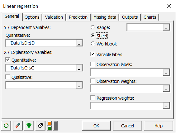
• Click on OK to run computation.

How to interpret the results of a simple linear regression in XLSTAT?

The first table displays the goodness of fit coefficients of the model. The R² (coefficient of determination) indicates the % of variability of the dependent variable which is explained by the explanatory variables. The closer to 1 the R² is, the better the fit is.

In this particular case, 60 % of the variability of the Weight is explained by the Height. The remainder of the variability is due to some effects (other explanatory variables) that have not been included in this analysis.

It is important to examine the results of the analysis of variance table (see below). The results enable us to determine whether or not the explanatory variables bring significant information (null hypothesis H0) to the model. In other words, it's a way of asking yourself whether it is valid to use the mean to describe the whole population, or whether the information brought by the explanatory variable(s) is of value or not.

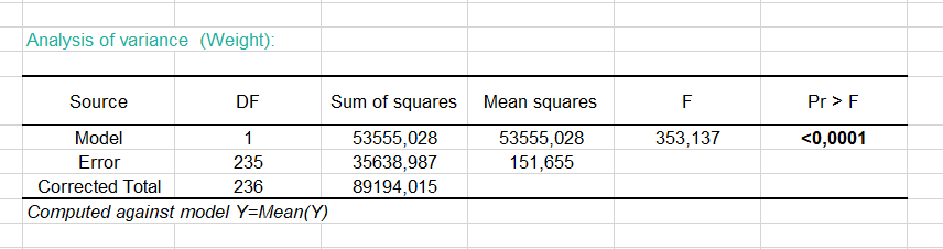
Given the fact that the probability corresponding to the F value is lower than 0.0001, we would be taking a lower than 0.01% risk in assuming that the null hypothesis (no effect of the two explanatory variable) is wrong. Therefore, we can conclude with confidence that the three variables do bring a significant amount of information.

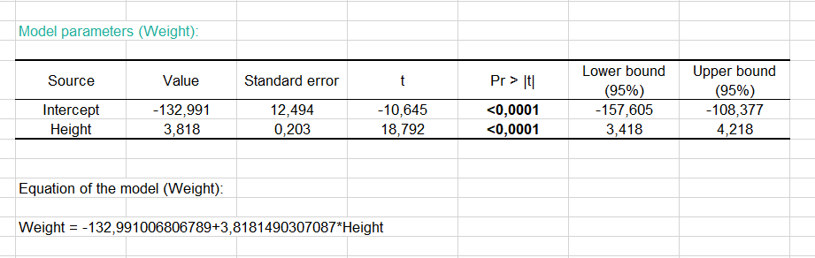
The following table gives details on the model. This table is helpful when predictions are needed, or when you need to compare the coefficients of the model for a given population with the ones obtained for another population. We can see that the 95 % confidence range of the Height parameter is very narrow, while the one for the intercept of the model is wider.

The equation of the model is written below the table. We can see that in the range of the variable Height that is taken into account here, when the Height increases by one inch, the Weight increases by 3.8 pounds.

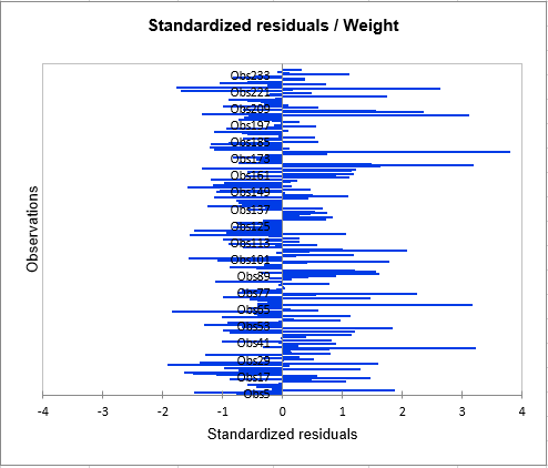
The next table shows the residuals. It enables us to take a closer look at each of the standardized residuals. These residuals, given the assumptions of the linear regression model, should be normally distributed, meaning that 95% of the residuals should be in the interval [-1.96, 1.96].

All values outside this interval are potential outliers, or might suggest that the normality assumption is wrong. We used XLSTAT's DataFlagger (Tools menu) to bring out the residuals that are not in the [-1.96, 1.96] interval. Out of 237, we can identify 9 residuals (38, 52, 69, 77, 108, 169, 179, 207, 224) outside the [-1.96, 1.96] range, an analysis that does not lead us to reject the normality assumption. A more detailed analysis of residuals can be found in the tutorial on ANCOVA .

The first chart (see below) allows us to visualize the data, the regression line (the fitted model), and two confidence intervals: the confidence interval on mean of the prediction for a given value of the Height is the one closer to the line.

The other one is the confidence interval on a single prediction for a given value of the Height. We can see clearly that there is a linear trend, but that there is a high variability around the line. We can also see that the 9 observations that are out side the [-1.96, 1.96] interval are outside the second confidence interval as well.

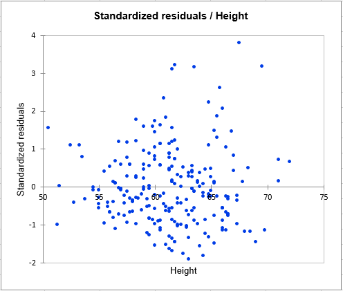
The third chart (see below) allows us to visualize the standardized residuals versus the Height. It is not the case here, but when plotting the residuals against the explanatory variable, if a trend is identified, this indicates that the model is not correct of there is an autocorrelation in the residuals, which is contrary to one of the assumptions of parametric linear regression.

The next chart allows to compare the predictions to the observed values. The confidence limits allow, as with the regression plot displayed above, to identify outliers.

The histogram of the residuals enables us to quickly visualize the residuals that are out of the range [-2, 2].

Conclusion of this linear regression in XLSTAT

The conclusion is that the Height allows us to explain 60 % of the variability of the Weight. A significant amount of information is not explained by the model we have used. In a tutorial on Multiple Linear Regression, the Age variable is added to the model to improve the quality of the fit.