Monotone regression / MONANOVA in Excel
This tutorial will help you set up and interpret a Monotone regression (MONANOVA) in Excel using the XLSTAT statistical software.
Monotone regression - Monanova method
Monotone regression and the MONANOVA method differ only in the fact that the explanatory variables are either quantitative or qualitative. These methods are based on iterative algorithms based on the ALS the algorithm (alternating least squares). Their principle is simple: it consists of alternating between an ordinary linear regression or ANOVA and a monotonic transformation of the dependent variables (after researching the optimal scaling).
The MONANOVA algorithm was introduced by Kruskal (1965). Monotonic regression methods and work on the ALS algorithm are due to Young et al. (1976).
These methods are commonly used as part of the full profile conjoint analysis. XLSTAT can apply them within a conjoint analysis but also independently.
The monotone regression tool (MONANOVA) combines a monotonic transformation of the response variable with a linear regression in order to improves the results of the regression.
Dataset for the MONANOVA method (monotone regression)
The data have been obtained in Lewis T. and Taylor L.R. (1967). Introduction to Experimental Ecology, New York: Academic Press, Inc.. They concern 237 children, described by their Gender, Age in months, Height in inches (1 inch = 2.54 cm), and Weight in pounds (1 pound = 0.45 kg).
Goal of this MONANOVA Analysis
Using the MONANOVA method, we want to find out how the weight of the children varies with their gender (a qualitative variable that takes value f or m), their height and their age, and to verify if a monotonic transformation improve the quality of the model.
Unlike a linear model, it combines a monotonic transformation of the dependent variable to an ordinary least squares regression. It is based on an iterative algorithm alternating between a general linear model (GLM) and a monotonic transformation to improve the quality of prediction.
Setting up a MONANOVA
After opening XLSTAT, select the XLSTAT- CJT - MONANOVA command, or click on the corresponding button of the XLSTAT-CJT toolbar (see below).

Once you've clicked on the button, the MONANOVA dialog box appears. Select the data on the Excel sheet. The Dependent variable (or variable to model) is here the Weight.
The quantitative explanatory variables are the height and the age. The qualitative variable is the gender. As we selected the column title for the variables, we leave the option Variable labels activated. The other options have been left at their default value.

The computations begin once you have clicked on OK. The results will then be displayed.
Interpreting the results of a MONANOVA analysis
The first table displays the goodness of fit coefficients of the model. The R² (coefficient of determination) indicates the % of variability of the dependant variable which is explained by the explanatory variables. The closer to 1 the R² is, the better the fit.
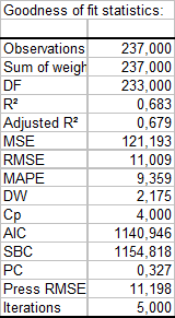
In this particular case, 68 % of the variability of the Weight is explained by the Height, the Age and the Gender. The remainder of the variability is due to some effects (other explanatory variables) that have not been or that could not be measured during this experiment. We can guess that some genetic and nutritive effects are involved.
As part of the MONANOVA method, an table of additional adjustment tests is displayed. These tests allow to obtain bounds on the p-value of the model.

It is important to examine the results of the analysis of variance table (see below). The results enable us to determine whether or not the explanatory variables bring significant information (null hypothesis H0) to the model. In other words, it's a way of asking yourself whether it is valid to use the mean to describe the whole population, or whether the information brought by the explanatory variables is of value or not.

The Fisher's F test is used. Given the fact that the probability corresponding to the F value is lower than 0.0001, it means that we would be taking a lower than 0.01% risk in assuming that the null hypothesis (no effect of the two explanatory variables) is wrong. Therefore, we can conclude with confidence that the three variables do bring a significant amount of information.
The following table gives details on the model. This table is helpful when predictions are needed, or when you need to compare the coefficients of the model for a given population with the ones obtained for another population. We can see that the p-value for the Gender parameter is 0.69, and that the corresponding confidence range includes 0. This confirms the weak impact of the Gender on the model. If we look at the parameter corresponding to Gender-f, it seems that for a given age and height, being a girl means a small increase of the weight.

The chart below provides analysis of the monotonic transformation performed.

We see that the transformation is close to the linear transformation. This leads us to compare the results with those of a linear model analysis of covariance (ANCOVA), the results associated with this analysis is available in sheet ANCOVA. We see that the R² is 0.63. This is lower than for the transformed model but the difference is not very important.
In conclusion, the size of the effect of the monotonic transformation does not provide much additional information on the quality of model prediction. The explanatory variables still have significant impacts and we can say that there is a linear relationship in the model.
Was this article useful?
- Yes
- No