Unit root (Dickey-Fuller) and stationarity tests on time series

This tutorial will help you set up and interpret unit root and stationarity tests - Dickey-Fuller, Phillips-Perron & KPSS tests - in Excel using XLSTAT.

Unit root and Stationarity tests

A time series Y_t (t=1,2...) is said to be stationary (in the weak sense) if its statistical properties do not vary with time (expectation, variance, autocorrelation). The white noise is an example of a stationary time series, with for example the case where Y_t follows a normal distribution N(mu, sigma^2) independent of t.

Identifying that a series is not stationary allows to afterwards study where the non-stationarity comes from. A non-stationary series can, for example, be stationary in difference (also called integrated of order 1): Y_t is not stationary, but the Y_t - Y_{t-1} difference is stationary. It is the case of the random walk. A series can also be stationary in trend.

Stationarity tests allow verifying whether a series is stationary or not. There are two different approaches: stationarity tests such as the KPSS test that consider as null hypothesis H0 that the series is stationary, and unit root tests, such as the Dickey-Fuller test and its augmented version, the augmented Dickey-Fuller test (ADF), or the Phillips-Perron test (PP), for which the null hypothesis is on the contrary that the series possesses a unit root and hence is not stationary. XLSTAT includes as of today 4 unit root tests: the Dickey-Fuller test, the ADF test, the PP test and the KPSS stationarity test.

Dataset for Unit root and Stationarity tests

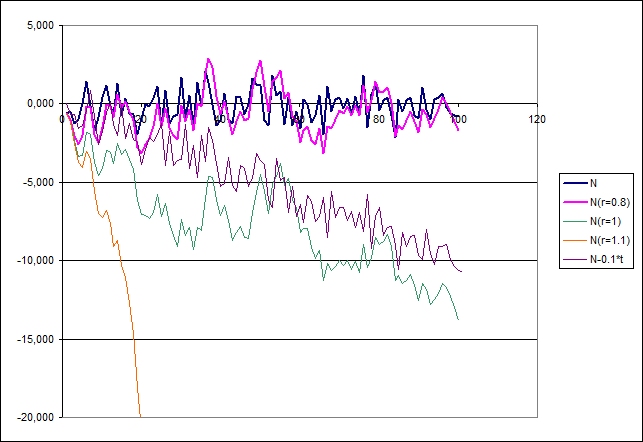
The data have been generated using a random N(0, 1) normal sample of 100 observations (series N), a stationary series built from that sample (series rho =0.8), an autocorrelated series (rho=1) and an explosive time series (rho=1.1), and a series that varies linearly with the time (N-0.1t).

Setting up the ADF, PP and KPSS tests on a time series

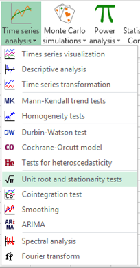
After opening XLSTAT, select the XLSTAT / Time / Unit root and stationarity tests command.

Once you've clicked on the button, the dialog box will appear. Select the data on the Excel sheet. In the “**Time series” field select the first and second time series.

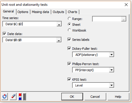
The option Series labels is activated because the first row of the selected data contains the header of the variable. The Stationary option is selected for the Augmented Dickey-Fuller test as the series does not exhibit an explosive characteristics. The Intercept model is chosen for the PP test as it seems the closest one to the time-series data generation process. The Level option is chosen for the KPSS test.

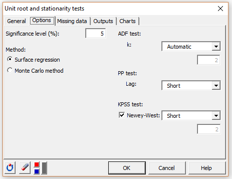
In the Option tab, you can choose among the two proposed options to estimate p-values and critical values for both unit root tests. The surface regression option uses the approach proposed by MacKinnon (J. G. MacKinnon, "Numerical Distribution Functions for Unit Root and Cointegration Tests", J.A.E., 1996) while the Monte Carlo option uses a predetermined number of simulations. The results of the test will then be displayed.

The computations begin once you have clicked the OK button.

Interpreting the results of an ADF test, a PP test and a KPSS test (example on stationary series)

After the summary statistics of the two selected series, the results of the ADF, PP and KPSS tests are displayed for the first, and then for the second series (see sheet Dickey-Fuller|Phillips-Perron1).

We can see that the three tests agree for these series. For the first series, both the ADF and the PP rejects the null hypothesis that the series is autocorrelated with (r=1) and retains the alternative hypothesis that it is stationary, and the KPSS test keeps the null hypothesis that the series is stationary.

For the second series, the p-values are not as low (ADF test) or high (KPSS test) as it was with the first sample but the same conclusions are retained.

Interpreting the results of an ADF test, a PP test and a KPSS test (example on non-stationary series)

We then run the three tests on columns E for which we know from our simulation parameters that the data generation process has a unit root. For every test, the unit root (or non stationarity for the KPSS test) is detected with a higher level of significance for the PP-test (see results on sheet Dickey-Fuller|Phillips-Perron2).

For the time series in columns F (see results on sheet Dickey-Fuller|Phillips-Perron3), we change the alternative option to explosive for the ADF test and to trend for the KPSS test. The KPSS tests lead to the conclusion that the series is not stationary while both unit root tests reject the hypothesis of a unit root in the data generation mechanism.

Interpreting the results of an ADF test and a KPSS test (example on a linear trend series)

We now run the tests on the last series that clearly exhibits a time trend (see results on sheet Dickey-Fuller|Phillips-Perron4). The Stationary option has been selected for the ADF test, the Intercept+Trend model for the PP test and the Trend version of the KPSS test. All three tests agree that the tested series is stationary once detrended.