Histograms and distribution fitting tutorial in Excel

The purpose of this tutorial is to generate a histogram and test if a sample follows a negative binomial distribution using the XLSTAT distribution fitting tool in Excel. This distribution is often used to represent the aggregation/dispersion phenomenon of bacteria in water environments.

Data to create a histogram and fit a distribution

The data correspond to an experiment where 200 samples of water from a river were cultured on medium with nutrients to determine the presence or absence of bacterial contamination with Escherichia coli. The number of colonies has been counted after 72 hours of incubation. In the Bact-Data column you will find the counts for the 200 samples.

Setting up the dialog box to create a histogram

Once XLSTAT is open, select the XLSTAT / Visualizing data / Histograms command (see below).

The dialog box then appears. Select the data on the Excel sheet named Data. In the general tab, select column B in the Data field. We activate the discrete option because the counts are discrete values. The Sample labels option is left activated because the first row of the data selection contains the name of the sample.

Click on the OK button to launch the computations. The results will then be displayed on a new sheet.

Interpreting a histogram

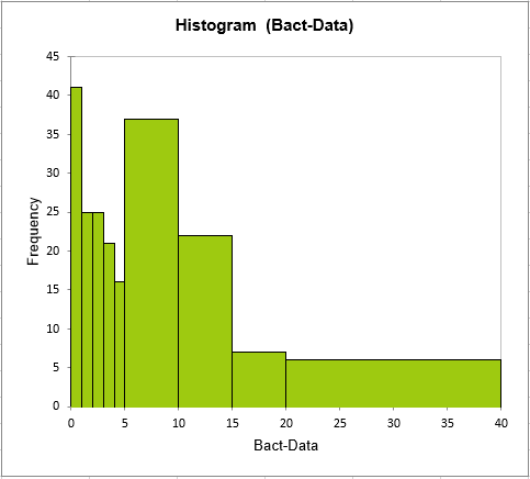
The histogram is displayed on the sheet Histogram below the Summary Statistics table and followed by a table where the statistics of the histogram are available.

On the histogram we can see that the most frequent value is 0, which represents over 20% of the data. That is, in more than one sample out of five, no bacteria has been found. We also notice that the frequency decreases quickly. In one sample, over 36 colonies have been counted. The following video shows how to do it.

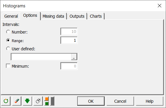
Creating a histogram specifying the bounds of the intervals

Since we want to test the fit between the negative binomial distribution function and the sample (the Chi-square test requires that there is are least 5 data in a class), and because of the uncertain precision of the counts of the bacteria, it seems necessary to group the counts into larger classes. For this reason, we create a list of bounds that seems coherent with our problem: 0,1,2,3,4,5,10,15,20,40. In order to verify if the frequencies of the new classes are greater than 5 and decrease regularly, we create a new histogram, specifying this time the bounds of the intervals in the tab Options.

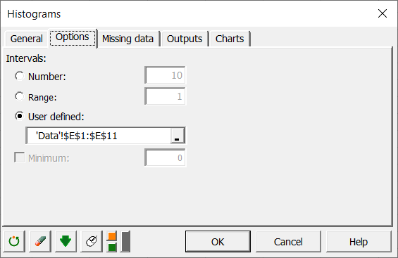The computations begin once you have clicked on the OK button, and the new histogram appears (see sheet "Histogram1").

The following video shows you how to reproduce those results.

As we are satisfied by this result, we can now use the distribution fitting tool to test if the sample follows a negative binomial distribution.

Setting up the dialog box to fit a distribution

Select the XLSTAT / Modeling data / Distribution fitting command (see below).

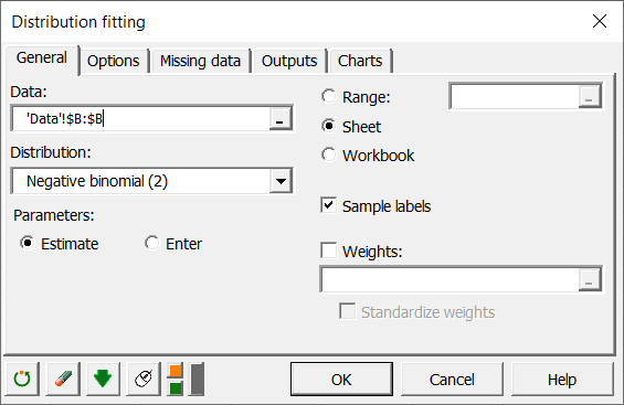
The Distribution fitting dialog box then appears. Select the data on the Excel sheet named Data.

In the General tab, select column B in the Data field. We let XLSTAT estimate the parameters of the negative binomial distribution function. XLSTAT offers two different formulations of the negative binomial distribution. The one that is adapted to our case is the second one.

In the Options tab, activate the Goodness of Chi-square tests, which is necessary to test our assumption. We use the bounds that we defined above.

Select the following options in the tab Charts.

Interpreting the results of a distribution fitting analysis

The first result of interest for us is the value of the k and p parameters of the negative binomial distribution (fitted using the maximum likelihood method), and the estimates of the sample and theoretical mean, variance, skewness and kurtosis. The closer these statistics obtained from the data and from the parameters, the better the fit. Here, the fit is excellent. Note: the theoretical mean is given by kp, and the variance by kp(p+1).

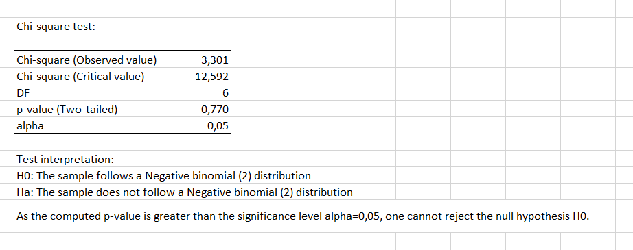
The Chi-square goodness of fit test allows to test if the Chi-square distance between the empirical and theoretical distribution functions is above a critical value or not. A visual comparison between the observed and theoretical frequencies is available on the next figure. 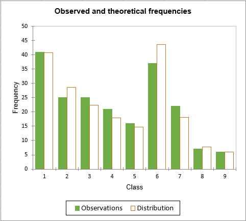For classes 2, 6 and 7, there seems to be a slight difference. In spite of this small difference, the p-value computed for the test (0.770) is significantly higher than the significance level we have chosen (0.05). Therefore, the Chi-square test confirms our hypothesis that the data follow a negative binomial distribution. As a conclusion, the presence of the bacteria of interest in the river in which the sample were collected, follows a negative binomial distribution (k=0.823, p=5.921), with a mean of 4.8 and a variance of 33.4.