Latent Semantics Analysis (LSA) in Excel tutorial
This tutorial explains how set up and interpret a latent semantic analysis n Excel using the XLSTAT software.
Dataset for latent semantic analysis
In this tutorial, we will use a document-term matrix generated through the XLSTAT Feature Extraction functionality where the initial text data represents a compilation of female comments left on several e-commerce platforms. The analysis was deliberately restricted to 5000 randomly chosen rows from the dataset.
Goal of this tutorial
The aim here is to build homogeneous groups of terms in order to identify topics contained in this set of documents which is described via a document-term matrix (D.T.M).
It is a simple and efficient method for extracting conceptual relationships (latent factors) between terms. This method is based on a dimension reduction method of the original matrix (Singular Value Decomposition). The latent semantic analysis presented here is a way of capturing the main semantic « dimensions » in the corpus, which allows detecting the main « subjects » and to solve, at the same time, the question of synonymy and polysemy.
Setting up a latent semantic analysis
Once XLSTAT is activated, select the XLSTAT / Advanced features / Text mining / Latent semantic analysis command:
 After clicking the button, the dialog box for the Latent semantic analysis appears.
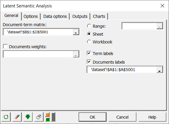
Select the data in the Document-term matrix field. The Documents labels option is enabled because the first column of data contains the document names. The Term Labels option is also enabled as the first row of data contains term names.
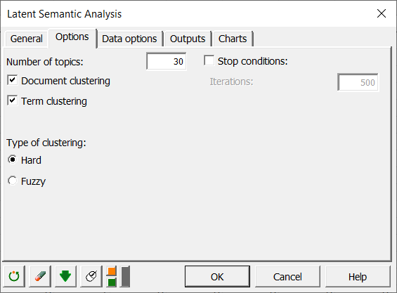
 In the Options tab, set the number of topics to 30 in order to show as many subjects as possible for this set of documents but also to obtain a suitable explained variance on the computed truncated matrix.
Choose to activate the options Document clustering as well as Term clustering in order to create classes of documents and terms in the new semantic space.
The Hard option forces each of the terms to belong to one andonly one topic at a time (the best semantic axis)
A Fuzzy classification, on the other hand, allows to have the same terms in several topics in order to capture polysemy (a term with several meanings).
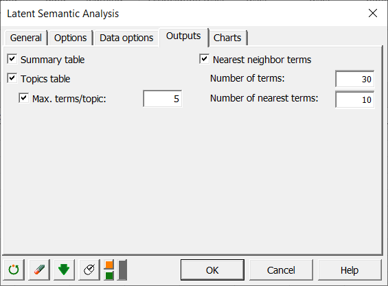
 In the Outputs tab, set the maximum number of terms per topic (Max. terms/topic) to 5 in order to visualize only the best terms of each topic in the topics table as well as in the different graphs related to correlation matrices (See the Charts tab).
The Nearest neighbor terms option is enabled to view the term-to-term correlations (cosine similarities) for each of the terms in the corpus.
The Number of terms is set to 30 to display only the top 30 terms in the drop-down list (in descending order of relationship to the semantic axes). The Number of nearest terms is set to 10 to display only the 10 most similar terms with the term selected in the drop-down list.
Interpreting a latent semantic analysis
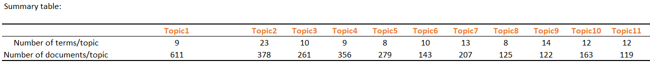
The summary table presents the total number of terms and documents per topic. The user is then able to display all the terms / documents in the correlation matrices and topics table as well.
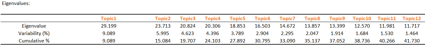
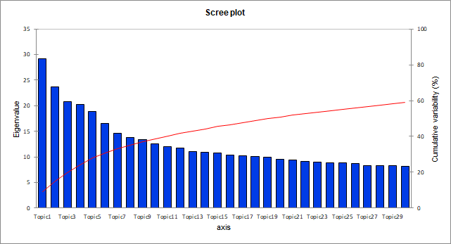
 The following table and graph are related to a mathematical object, the eigenvalues, each of them corresponds to the importance of a topic.
The quality of the projection when moving from N dimensions (N being the total number of terms at the start, 269 in this dataset) to a smaller number of dimensions (30 in our case) is measured via the cumulative percentage of variability.
Each eigenvalue therefore corresponds to a topic and here we see that a dimension set to 30 enable to obtain a total cumulative variability of approximately 60% of the original matrix.
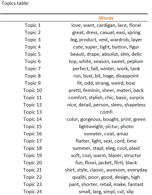
 The table below lists the best terms for each of the topics found. These are displayed in descending order of importance with the topic in question. This first result highlights classes of elements often associated with positive or negative feelings about particular aspects of clothing purchased online.
For example, topics 8 and 24, composed of term pairs {small, large} and {run, bust}, relate to size problems on clothing lines. These pairs can therefore be combined to become a common term that symbolizes this size issue and thus eliminate semantic redundancies (synonymy) in the initial document-term matrix.
Topic 6 makes a statement of success by associating a positive sentiment {sweet} with a clothing lines {top, peplum}.
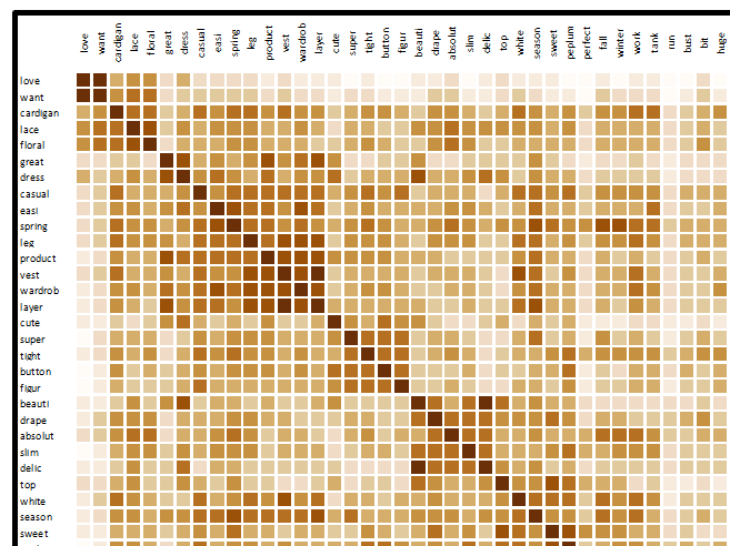
The relationship strength for term pairs is represented visually via the correlation graph below. It allows visualizing the degree of similarity (cosine similarity) between terms in the new created semantic space. The cosine similarity measurement enables to compare terms with different occurrence frequencies.
The similarities are between 0 and 1, the value 1 corresponding to a perfect similarity or dissimilarity (similarity in case of agreement and dissimilarity in case of disagreement).
Terms are displayed in the order of detected topic classes (these classes can also be viewed by enabling the « Color by class » option on the Charts tab).
 The two examples below show similarities between terms closest to the selected terms (top and run here) in the drop-down list, in descending order of similarity.

 To conclude, here is a quick application of latent semantic analysis which shows how to create classes from a set of documents which combine terms expressing a similar characteristic (clothing size for example) or feeling (negative or positive). In order to apply a dimensional reduction on the input DTM matrix and to keep a good variance (see eigenvalue table), you can retrieve the most influential terms for each of the topics in the topics table. This allows you to later apply a more efficient learning algorithm.
Was this article useful?
- Yes
- No