Univariate Clustering in Excel, tutorial
This tutorial shows how to set up and interpret a univariate clustering in XLSTAT.
Univariate clustering is a statistical method that aims to cluster N unidimensional observations, described by a single quantitative variable, in K homogeneous groups (clusters).
Dataset for univariate clustering
The data represent the grades of 29 students in 8 subjects: Mathematics, Chemistry, English, French, Physics, History, Physical Education and Spanish. The grades vary from 0 to 20. Each row corresponds to a student and each column to a subject.
Our goal is to create five homogeneous study groups based on the students' performance for each subject.
Setting up a univariate clustering with XLSTAT
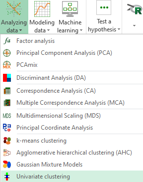
Once XLSTAT is open, select Univariate Clustering in the Analyzing data menu.
The Univariate clustering dialog box appears.
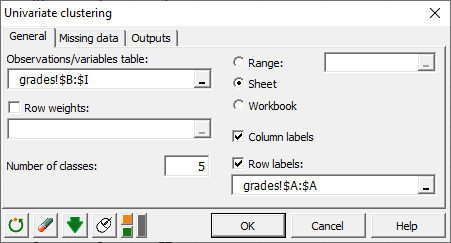 In the General tab, select the Observations/variables table which contains the grades per student and per subject (columns B to I).
Here, the rows do not have distinct weights (or importance) because no student is more significant than another when making the groups. Thus we should not use the Row weights option.
The number of classes refers to the number of groups to create per subject. In our example, we set it to 5 groups.
Finally, we check Column labels (because we have specified the subject labels). We also check and specify the Row labels (student id). Here, it is column A.
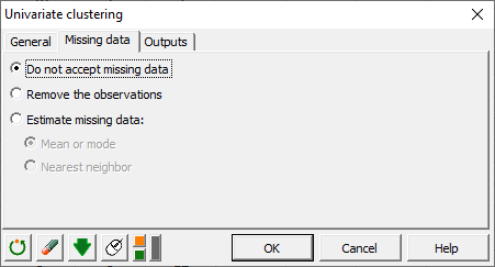 In the Missing data tab, we choose not to accept missing data as we expect all students to have a grade per subject.
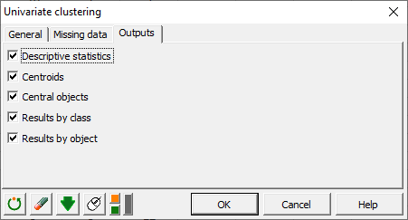 Finally, in the Outputs tab, we check all proposed outputs. Once we've clicked on OK, the calculations start and the results are plotted.
Interpreting the results of a univariate clustering with XLSTAT
Univariate clustering returns several tables in the output sheet. First of all, a descriptive table is displayed summing up the raw data.
 For each variable, we have 29 observations. There is no missing values. We can also see the maximum, minimum, mean and standard deviation for each subject. For example, the class mean for mathematics is situated at 9.69. The standard deviation is 5.594, which means that most of the grades are approximately between 4.1 et 15.3.
Since we are running a univariate clustering, the analysis is done independently for each subject. Let's interpret the results regarding mathematics.
First of all, we may suggest that all subjects are well distinct given the different values of the initial class centroids.
 After running the clustering, the centroids have not changed. In the same table, the sum of weights is also displayed which equals to the number of individuals per class as well as the within-class variance. Here, the most homogeneous class is class 3 because it has the smallest within-class variance. Hence, the less homogeneous class is class 5.
  Then, we have a table summing up the distances between the class centroids. Classes 3 and 5 are 16 points away from each other. Indeed, the centroid (or mean grade) of class 3 is 2.17 while the centroid of class 5 is 18.25.
 We can also study the central objects (students) of each class, having gotten the median grade, in a similar way. Student 6 (center of class 3) has gotten 2/20 in mathematics while student 19 (center of class 5) has gotten 19/20, which shows once more the gap between classes 3 and 5.
 Now, let’s have a look at the detailed results for each class as well as the students. Each study group has between 4 and 7 students. As seen before, intra-class variance indicates that group 3 is the most homogeneous while group 5 is the least homogeneous. The minimal, maximal and average distances to centroid give us information regarding the results of each student present in each group in comparison to the average grade per group. In group 1, the students have on average 0.77 points more or less than the average grade of the group.
Finally, we have the lists of the students composing each group. For instance, group 2 contains students 3, 4, 7, 9, 14 and 23. This is coherent if we look at the raw data: the average grade of group 2 is 6. Students 3, 4, 7, 9, 14 and 23 have scored 6, 6, 5, 6, 8 et 5 out of 20.
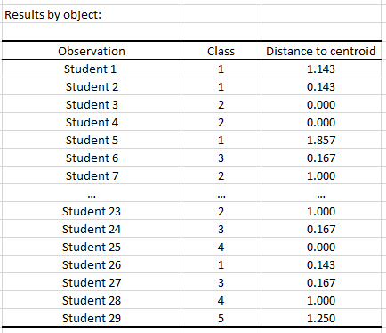
 Finally, the Results by object table sums up the study groups (classes) to which each student belongs as well as how far their grade is from the average grade of the group (=distance to centroid).
Conclusion of a univariate clustering analysis
Univariate clustering enabled us to cluster students into homogeneous study groups for each subject independently.
Not sure which clustering method to use? Check out our guide and learn how to choose the most appropriate clustering method accordging to your data.
Was this article useful?
- Yes
- No