Ordinale Logit-Modelle in Excel - Anleitung

This tutorial shows how to set up and interpret an Ordinal Logit model in Excel using the XLSTAT software.

Principles of Ordinal logit model

The ordinal logit model consists of an alternative to the classical logit model for variables to be explained by ordered modalities (this method can also be called ordinal logistic regression). It allows to model the cumulative probability that an event occurs given the values of a set of quantitative and/or qualitative descriptive variables.

The purpose of this model is as follows: we want to understand or predict the effect of a series of variables on an ordered qualitative response variable. We can thus understand the impact of the choice of a modality according to the explanatory variables by taking into account the order of the modalities. This model is based on cumulative probabilities.

Ordered logit model can be helpful to model the effect of some descriptive variables on the satisfaction with respect to a brand in a market. The dialog box for running a logit model is the same as the one used for binary logistic regression or multinomial logistic regression.

Dataset for running an ordinal logit model

Our example examines the factors that influence the decision to apply or not to for a higher education course. High school students are asked whether they will "unlikely," "somewhat likely," or "very likely" apply to a university. Thus, our response variable has three categories. The explanatory data are the parental education level, the status of the undergraduate institution, and the average grade of the high school student surveyed.

The researchers have reason to believe that the "distances" between these three points are not equal. For example, the distance between "unlikely" and "somewhat likely" may be shorter than the distance between "somewhat likely" and "very likely". This leads us to use an ordinal logit model rather than an ANCOVA, assuming that the 3-way variable can be treated as a quantitative variable.

Setting up an ordinal logit model in XLSTAT

To open the Ordinal Logit Model dialog box, select the XLSTAT / Modeling data / Logistic regression feature. Once you have clicked on the button, the Logistic Regression dialog box appears.

The ordinal logit model is activated by selecting the Ordinal option as the response type. The Response variable corresponds to the column in which the variable to be explained is located.

There are two qualitative explanatory variables; the type of high school (private/public) and the parents' education level. There is a quantitative explanatory variable: the average grade obtained in high school. As we have selected the variable labels, we need to select the Variable labels option.

Many other options are available in the other tabs of the dialog box (for more details, see the XLSTAT help).

Once you have clicked on the OK button, the calculations are performed and the results displayed.

Interpreting the results of a ordinal logit model

The goodness-of-fit statistics table gives several indicators of the quality of the model (or goodness of fit). These results are equivalent to the R² of the linear regression and the ANOVA table. The most important value is the Chi² associated with the Log ratio (L.R.). It is the equivalent of Fisher's F-test of the linear model: we try to evaluate if the variables provide a significant amount of information to explain the variability of the response variable. In our case, as the probability is lower than 0.0001, we may conclude that the variables bring a significant amount of information. The model parameters table gives the first details about the model and helps us evaluate the contribution of the variables to the quality of the model. It is somewhat different from the multinomial logistic regression. Indeed, if we have a constant for each modality of the response variable (university inscription here), the coefficients of the explanatory variables are common to each modality. 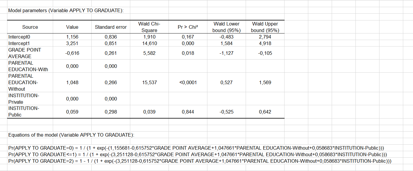We can therefore conclude that the higher the average grade, the higher the probability of going to university. In fact, the coefficient is significantly negative, and our model has as reference modality 2 (university inscription). Therefore, a negative coefficient in the prediction of the 0 and 1 modalities indicates that the higher the mean, the less likely the 0 and 1 modalities occur. Furthermore, given the probability associated with the Chi-square tests, we can see that the variable that most influences students' choice is their parents' education level. On the other hand, the status of the school does not have a significant influence.

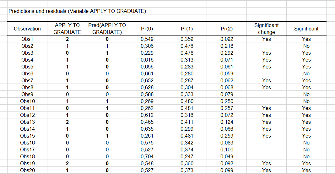
Next, you can view the Predictions and Residuals table. We can see that the first high school student (Obs1) is willing to apply to a university (modality 2) but the model predicts that he will probably not apply (modality 0). Indeed, we can see that the probability of modality 0 ("unlikely") is the highest with value 0.549 while the probabilities of "somewhat likely" or "very likely" modalities are estimated at 0.359 and 0.092 respectively.

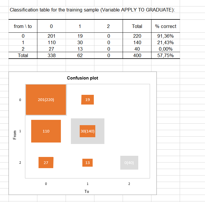
The column Significant change indicates that the change in value between the predicted modality and the observed one is significant. The second column, Significant, indicates whether the probability of the predicted modality is higher than the ones of the others. Note that these two columns appear if the Significance analysis option has been checked in the dialog box outputs. The classification table for the training sample (sometimes called the confusion matrix) helps us visualize the percentage of well classified observations for each modality (true positives and true negatives). For example, observations of the "unlikely" modality were correctly classified (91.36%) while the observations of the "somewhat likely" modality were correctly classified at only 21.43%. Finally, none of the observations of the modality "very likely" (code 2) were well classified.

The confusion plot allows to visualize the above table in a synthetic way. The grey squares on the diagonal represent the observed numbers for each modality. The orange squares represent the predicted numbers for each modality. We can see that the surfaces of the squares overlap almost completely for the "unlikely" modality (code 0), unlike the "somewhat likely" modality (code 1) or the "very likely" modality (code 2). In other words, for the modality "unlikely" (code 0), the model has predicted 201 observations out of 220 observed observations.