Bland Altman plot to compare methods in Excel

This tutorial will show you how to draw and interpret a Bland Altman plot to compare methods in Excel using the XLSTAT statistical software.

Method comparison with the Bland Altman method

When developing a new method to measure the concentration or the quantity of an element (molecule, micro organism, …) you might want to check whether it gives results that are similar to a reference or comparative method or not. If there is a difference, you might be interested in knowing if this is due to a bias that depends on where you are on the scale variation. If a new measurement method is cheaper than a standard, but if there is a known and fixed bias, you might take into account the bias while reporting the results. XLSTAT provides a series of tools to evaluate the performance of a method compared to another.

Dataset for method comparison with the Bland Altman method

The data correspond to a medical experiment during which the concentration of an antibody is measured for 8 mice submitted to 8 different doses of a new molecule being tested. For each mouse, a blood sample has been taken and divided into four homogeneous sub-samples. Two methods are being tested each on 2 of the 4 sub-samples. The first method is currently considered as the reference, but it is much more expensive than the second and new method.

Our goal is to check if it is possible to use the new method instead of the reference one.

Setting up a Bland Altman method

• After opening XLSTAT, select the Laboratory data analysis/Method Comparison (Bland Altman...) feature

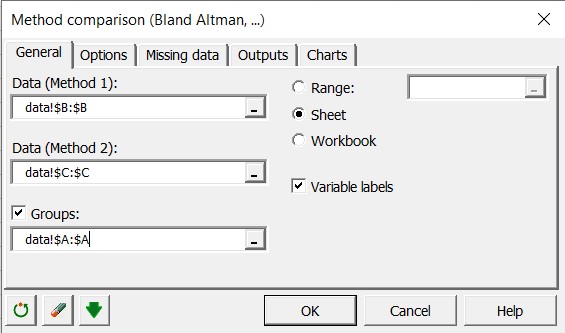
• When you click on the button, a dialog box appears. Select the data that correspond to the first method, then to the second method. As the experiments have been replicated, we need to specify the mouse ID in the first column and select it.

• In the Options tab, we do not select the Difference plot option as the Bland Altman plot is already a type of difference plot. In the other tabs the options are left unchanged.

• When you click OK, the computations are done and the results are displayed.

Interpreting the results of a Bland Altman method

The first table displays the descriptive statistics for the two methods. The new method has a larger mean but a larger variance as well.

Then, the repeatability of the methods is calculated. To evaluate the repeatability of a method, one needs to have several replicates. We have here two replicates per method for each mouse. If a method is repeatable, the variance within the replicates should be low. XLSTAT computes the repeatability as a standard deviation and displays a confidence interval. Ideally, the confidence interval should contain 0.

We see here that for both methods the standard deviations are low compared to the total standard deviation, but their confidence intervals do not include 0. For the 7th mouse, there is a strong difference between the two measures for the reference method. This might be due to a measurement error or to a problem with the sample. This should be investigated further.

Next, we have the results of the Student t test, performed on the means for each mouse. This test basically computes for each mouse the difference between the two methods, and checks whether it is different from 0 or not. This test requires the assumption that the differences are normally distributed. Using a normality test, one can check this. However, we have only 8 data here and the result of the normality tests (that confirm the normality) are not very reliable.

We see that in our case, the p-value is 0.02, meaning that the risk of concluding that the methods are different while they would not be is low. We could stop the analysis here, but we want to investigate further the difference and not only take the decision on the basis of a test that requires assumptions we are unsure of.

The first plot allows to quickly see if there is a fixed bias or not, by comparing directly the new method (ordinates) to the reference method (abscissa). The line on the plot is the identity line (or bisector). In an ideal case where the two methods would give exactly the same results, the data would be on that line.

In our case we see that 5 of the 8 points are above the identity line. This is nothing surprising, but as the 3 points that are below are closer to the line, we suspect a positive bias (a bias means that there is by nature a difference between the methods).

The Bland Altman analysis starts with an analysis of the bias. It's estimate is 0.744, with a 95% confidence interval that does not include 0. This confirms our first guess.

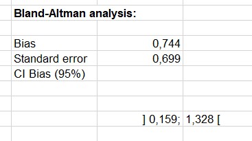
The next confidence interval on the differences is a confidence interval around the bias for an individual difference (the bias being the mean of the differences). This means that if the difference is normally distributed and if the bias has the value we assume, a difference between two measures should lie in this confidence interval.

Theses results and the differences themselves are plotted against the average of the measures obtained from the two methods. We obtain the Bland Altman plot. We see here a strange sinusoidal pattern which is probably a matter of chance. But this could be investigated further.

The Pearson correlation coefficient is computed with a confidence interval to check whether the correlation between the difference and the average is different from 0 or not. Not surprisingly, the correlation is not significantly different from 0. If the methods were similar if if the bias was constant the correlation should not be different from 0.

Last, the box plot and the histogram of the differences are displayed for those who would like to check the normality assumption visually. While the histogram is of little interest for so few data, the box plot shows that the median and the mean are quite far from each other, but again, we have only few data here.

As a conclusion, it is very likely that there is a bias. This does not make the new method not relevant, if the bias is understood and constant for the scale that is being used. This should be further investigated through complementary experiments.