Life table analysis in Excel tutorial
This tutorial will show you how to set up and interpret a life table in Excel using the XLSTAT statistical add-on software.
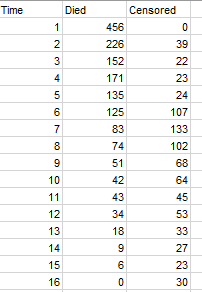
Dataset to generate a life table
The data have been obtained in [Lee E.T. (1992). Statistical Methods for Survival Data Analysis, Second Edition, John Wiley & Sons, New York] and represent the evolution of the number of patients with angina pectoris, during a 15 year period (Jan 1,1927 - Dec 31,1941).
Survival time is measured as years from the time of diagnosis. The counts correspond to events (number of patients who died during a time interval) and to withdrawals (number of patients lost to follow up).
Our goal is to determine to display the life table, analyse the median residual lifetime (or median survival time), and plot the non parametric estimate of the survival distribution function.
Setting up a life table analysis
After opening XLSTAT, select the XLSTAT / Survival analysis / Life table analysis command.
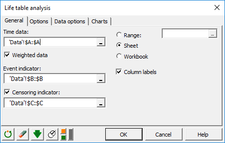
 Once you've clicked on the button, the Life table analysis box will appear. Select the data on the Excel sheet. The Time data corresponds to interval end times.
As the data correspond to counts, check the Weighted data option, and then select the "Died" data in the Event indicator field, and the "Censored" data in the Censored indicator field.
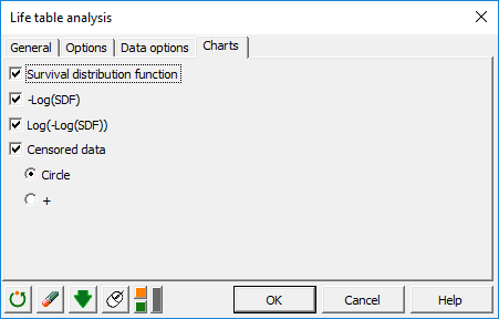
 In the Charts tab, activate the charts you wish to display, and choose the symbol you want to use to represent Censored data.
The computations begin once you have clicked on OK. The results will then be displayed.
Interpreting the results of a life table analysis
The first table displays a summary of the data. The next table corresponds to the "Actuarial table". It contains the results of the life table analysis, including several key indicators such as the median survival time.
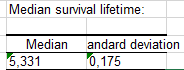
 The third table isolates the median survival time and its standard deviation. From these values we can conclude that the median residual lifetime for angina pectories is 5.3 years. In other words, out of 100 patients, 50 would be dead 5.3 years after having contracted the disease.
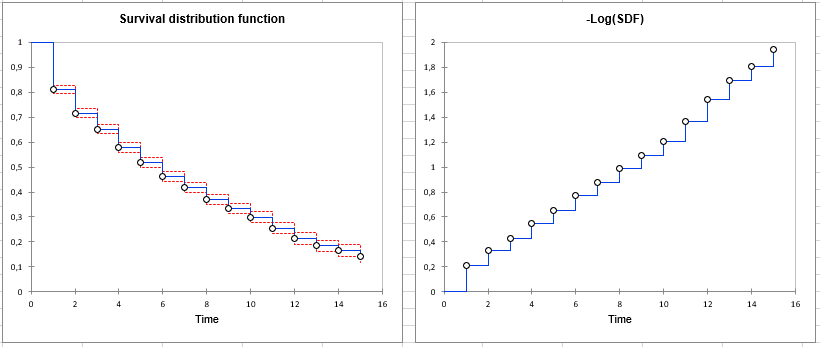
 Last, we can visualize several curves, including the the survival distribution function (SDF, or survivor function), and the -Log(SDF) curve. From the latter, we see that the function is close to an exponential model.
Was this article useful?
- Yes
- No