X-13ARIMA-SEATS Seasonal Adjustment in Excel

This tutorial shows how to run and interpret the X-13ARIMA-SEATS procedure using the XLSTAT-R engine in Excel.

Dataset to fit the X-13ARIMA-SEATS procedure

This dataset represents the United States unemployment level (thousands of persons) since January 1990 to November 2016, month by month. Here is the source for this dataset: U.S. Bureau of Labor Statistics, retrieved from FRED, Federal Reserve Bank of St. Louis; https://fred.stlouisfed.org/series/LNU03000000, December 14, 2016.

Goal of this tutorial

The goal of this tutorial is to set up an X13-ARIMA-SEATS procedure on this dataset, to identify a trend, and to predict the United States unemployment level in the future.

The X13-ARIMA-SEATS function developed in XLSTAT-R calls the seas function from the seasonal package in R (Mike Toews).

Setting up an X-13ARIMA-SEATS procedure in XLSTAT-R

Select the XLSTAT-R/seasonal/Arima x13(seas) Command (see below).

The X-13 Arima dialog box appears.

In the General tab, select column B (unemployment level) for the Time Serie field. Then select column A into the Date data field. The Period field corresponds to the number of observations per unit of time. Here, we select 12, as we are working year by year, with a single observation per month. The Custom model parameters allows you to fill your own model parameters. Here, we choose not to activate it thus the X-13ARIMA-SEATS procedure will automatically compute the parameters.

In the Options tab, you can either check or not the options to automatically detect the outliers, compute the model on your log-transformed data, or detect trading days and Easter effects with AIC tests. You have also the possibility to choose the x11 procedure rather than the X-13ARIMA-SEATS. Here, we retain the X-13ARIMA-SEATS procedure for the computations.

Interpreting the results of X-13ARIMA model

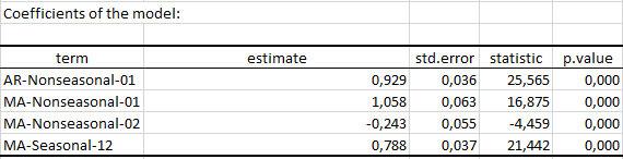
The first table shows the estimated model coefficients with their pvalues.

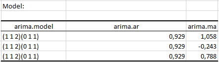
The following table represents the chosen model parameters for the procedure. Here, the X-13ARIMA-SEATS procedure retained the following model (p=1 d=1 q=2) (P=0 D=1 Q=1).

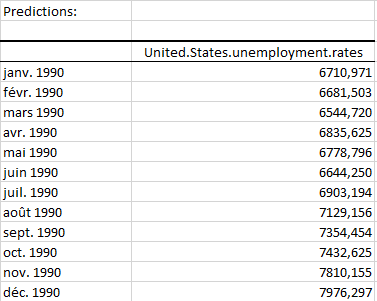
The third table displays the predictions of the initial time serie based on the fitted model.

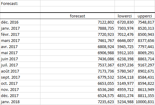
Finally, the last table shows the forecasted values with lower and upper bounds.

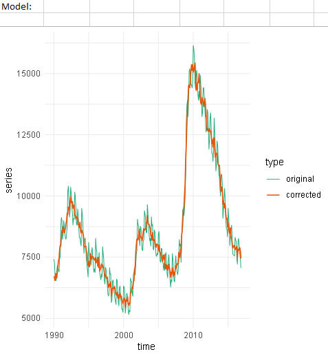
A graph is also available showing the original and the corrected time serie based on the X-13 model.

You will find a tutorial which explains more in detail how to set up and interpret an ARIMA in general. Click here , to read more.