Surface response design in Excel tutorial
This tutorial explains how to calculate and interpret a response surface design with Excel using XLSTAT.
Dataset for the analysis of a response surface design
An Excel workbook including both the data used in this example and the results obtained can be downloaded by clicking on the link above.
The data come from a classic example described in [Louvet, F. et Delplanque L. (2005). Design Of Experiments: The French touch, Les plans d’expériences : une approche pragmatique et illustrée, Alpha Graphic, Olivet, 2005]. An experimental design to analyze a 2-factors response surface is used to graphically represent this surface and analyze it.
Goal of this tutorial
Response surface designs are used to analyze problems in which a response is influenced by several variables and for which the objective is to optimize that response.
Note: Screening designs, on the contrary, are used to analyze the factors and not to optimize the response.
In this tutorial, we will find the optimum value of debinding temperature (F1) and debinding time (F2) of an industrial process in order to extract the binder in the field of ceramics. We seek to obtain a maximum percentage of extracted binder.
Setting up the dialog box for generating a surface response design
After launching XLSTAT, click on the DOE button on the XLSTAT bar and select response surface design.
The dialog box pops up.
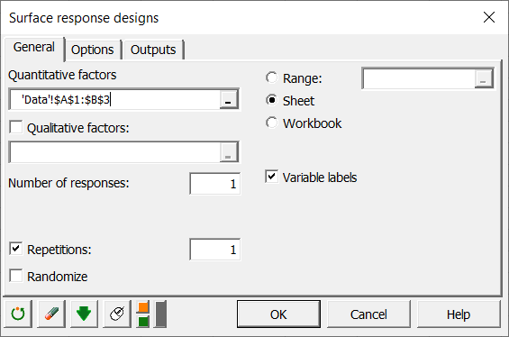
In the General tab, select the table of quantitative factors (this table must contain a maximum of two rows, the minimum and the maximum for each of the factors), as well as the number of responses (1).
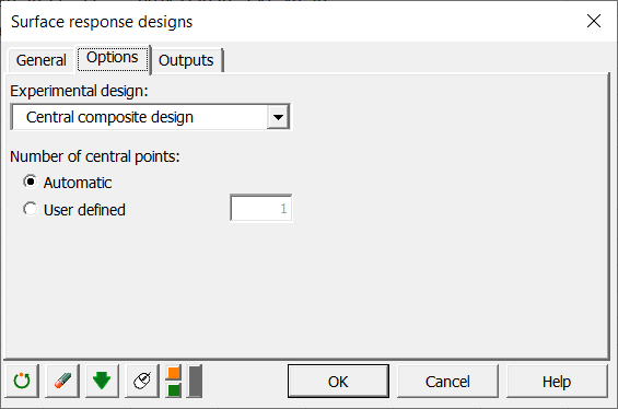
In the Options tab, select a central composite design as the type of design.
Then click on the OK button, the calculations begin.
Results of the generation of the experimental design
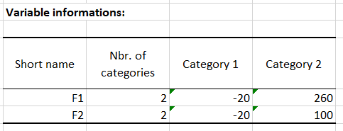
A table with all the information associated with the factors is displayed.
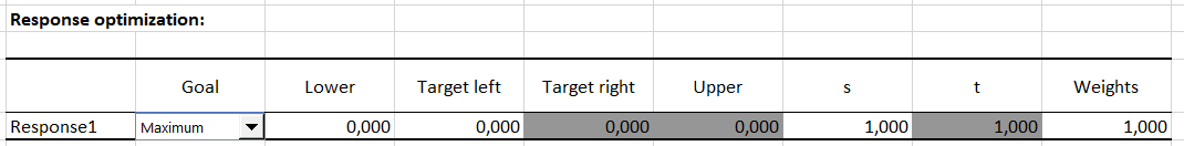
Then the design is displayed, in which you need to fill the last column, corresponding to the response, with the results of the experiments. Below, the response optimization table is displayed, it will automatically fill in after entering the response results.
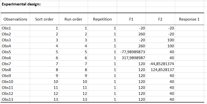
Once the design has been generated, we therefore carry out the 13 experiments and enter the results in the appropriate column in the table of the design.
Then select the option to maximize the response in the optimization table, which will find the optimum values of debinding temperature (F1) and debinding time (F2) of the industrial process to obtain a percentage of maximum extract binder.
In the workbook used for this tutorial, the results are already present, they have been highlighted in yellow in order to quickly identify them.
Setting up the dialog box for the analysis of the experimental design
You then have two options to start the design analysis.
- The first is simply to click on the launch analysis button located below the design generated previously. This first solution makes it possible to automatically fill in the fields of the dialog box.
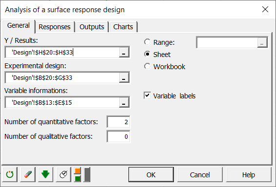
- The second is to click on the DOE button on the XLSTAT bar and select analysis of a response surface design.
Once you click on the button, the dialog box appears. If the box is not pre-filled, select, in the general tab, the column with the results of the experiments, the design of the experiments and the variable information table. Be careful to select all the columns of the design so that the analysis works.
In the Options tab, check the responses optimization option and select the corresponding table, taking the column headings well.
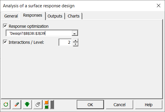
Once you've clicked OK, the calculations begin. A new dialog box appears in order to choose which terms we want to use in the analysis. Select all the terms in order to have the terms of the quadratic model.
Interpret the results of the surface response design analysis
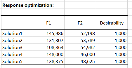
A first table is displayed, providing the results of the responses optimization. This shows us several effective solutions to obtain a maximum percentage of extracted binder. According to this table, it is therefore necessary to have a debinding temperature of around 135°C and a debinding time of around 52 minutes.
Then all the results of the analysis of variance are displayed, starting with the goodness of fits coefficients. We can see that the R² = 0.996, which shows that the regression describes the data very well.
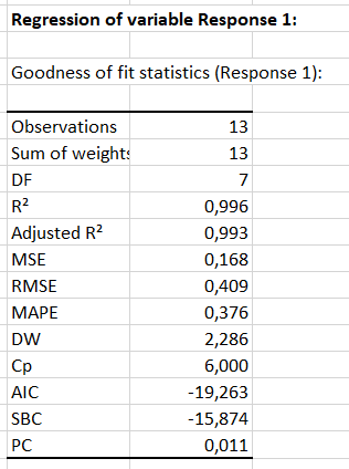
Further details are available in the rest of the results, notably with the model parameters and the model equation.
Then the response surface is displayed. This is possible thanks to contour graphs in 2 and 3 dimensions (2D and 3D). We can clearly see that the optimal surface is in red in these graphics.
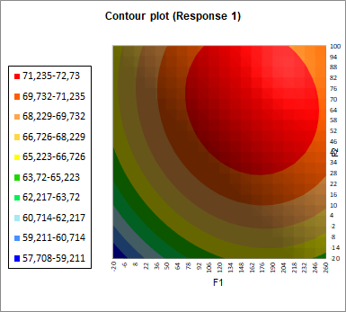
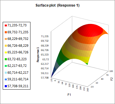
The optimum is around 135 degrees Celsius and 52 minutes. The value of the response variable at this point is greater than 72.4%.
Was this article useful?
- Yes
- No