Kolmogorov-Smirnov test in Excel tutorial
The data correspond to scores (0 – 30) measuring the quality of two brands of shoes (brand A and brand B). Scores were computed based on a survey addressed to customers using either brand. 15 customers have answered for brand A and 8 different clients for brand B.
Goal of this tutorial
This tutorial is divided into two parts:
In the first part we compare the distributions of the two samples without making assumptions on underlying theoretical distributions (normal distribution for example). We use the non-parametric Kolmogorov-Smirnov test, which is well suited in this case.
In the second part, we use the Kolmogorov-Smirnov test to compare the distribution of one sample to a theoretical distribution.
Part 1: Running a Kolmogorov-Smirnov test to compare two observed distributions in Excel
Here, we are interested in comparing the distributions of the two samples.
First of all, what do these distributions look like? Histograms are a good tool to visualize continuous distributions: XLSTAT / Visualizing data / Histograms.

In the General tab, select both samples inside the Data cell range. In the Options tab, activate the minimum option and enter 0 in the box. This will force histograms to have the same lower bound on the x axis making their comparison easier. Click on the OK button.

The histograms appear in the results sheet:

Without making any theoretical assumption, we may say that the distribution of sample B is more skewed towards low values compared to the distribution of sample A. We will now use the Kolmogorov-Smirnov non-parametric test to compare the two distributions. Go to XLSTAT / Nonparametric tests / Comparison of two distributions.


Select the Brand A column in Sample 1 and the Brand B column in sample 2. The Kolmogorov-Smirnov test allows samples to be unbalanced such as in our data: sample B contains fewer scores than sample A. In the Options tab, notice it is possible to select a one-tailed alternative hypothesis and/or an exact computation of the p-value. In the Charts tab, activate the Cumulative histograms option. Click on the OK button.
The results sheet contains the Kolmogorov-Smirnov statistic (0.475) that can be easily extracted (see further, the cumulative histograms chart). This statistic is associated to a p-value (0.190) indicating that the two distributions are not significantly different at alpha = 0.05.
Confused with p-values and statistical significance? Do not hesitate to visit our tutorial.

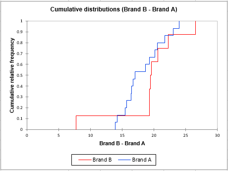
The cumulative distributions chart presents the studied variable (survey scores) on the x axis. For a given point on the x axis, a brand’s cumulative relative frequency is the proportion of scores smaller than this point among the scores of the brand. Thus, as previously suggested by the histograms, brand B seems to start cumulating scores earlier than brand A along the x axis. Let’s take a look at the medians, which are the scores corresponding to a cumulative relative frequency of 0.5. The median score for brand B (~20) seems to be higher than the median score for brand A (~17).
Kolmogorov-Smirnov’s D test statistic is the highest deviation occurring between the two curves.
It is calculated by the following formula:
where F_n and F are the distribution functions.
In our example, this deviation value falls inside the median region, but this may not necessarily be the case when using other data. The higher the D statistic, the lower the p-value and the more significant the difference between the two distributions.
Part 2: Running a Kolmogorov-Smirnov test to compare an observed distribution to a theoretical one in Excel
Suppose that the quality scores of brand A were obtained in France. For US customers, this score follows a normal distribution with a mean of 21.5 and a standard deviation of 2.3. We may ask ourselves if the French scores distribution is significantly different from the theoretical distribution of the US scores.
Here again, we will use the Kolmogorov-Smirnov test. The only difference with the previous part is that we aim at comparing an observed distribution to a theoretical one instead of comparing two different distributions.
To run the test, go to XLSTAT / Nonparametric tests / Distribution fitting.

In the General tab, select the brand A data, the normal distribution, activate the Enter option and enter the following parameters: µ = 21.5 and sigma = 2.3. In the Charts tab, activate the Cumulative histograms option. Click on the OK button.

In the results sheet, the histogram (on the left below) shows that the observed distribution of our data lays on low score values compared to the theoretical curve reflecting the US scores distribution (red line).


The Kolmogorov-Smirnov test is associated to a p-value of 0.000 suggesting that the null hypothesis should be rejected and that the observed distribution is significantly different from the theoretical one at alpha = 0.05.
Not sure that you have chosen the right test? This will let you know.
Was this article useful?
- Yes
- No