Repeated measures ANOVA in Excel tutorial
This tutorial will help you set up and interpret a Repeated Measures ANOVA in Excel using the XLSTAT software.
Dataset for running a repeated measures ANOVA
The data correspond to an experiment in which a treatment for depression is studied. Two groups of patients (1: control / 2: treatment) have been followed at five different times (0: pre-test, 1: one month post-test, 3: 3 months follow-up and 6: 6 months follow-up). The dependant variable is a depression score.
We have performed repeated measures ANOVA in order to determine the effect of the treatment and the effect of time on the depression score. The repeated measures ANOVA model is the same as the classical ANOVA model with interactions:
![]()
We have one fixed factor (group), one subjet factor (the patients) and the repetition. The interaction between the group and the repetition is included in the model.
The difference between classical ANOVA and repeated measures ANOVA is that measures on the same patient at different times are not supposed to be independent and, thus, the covariance matrix of the errors is not diagonal.
Goal of this tutorial
In this tutorial, we use the least squares estimation method (LS) to estimate the model. The variance-covariance matrix is supposed to be spherical.
This method is very simple: First, a classical ANOVA is performed on each time measured. Results are the same as in a classical analysis of variance. Then, results based on the covariance matrix and on the repetition factor are given.
You can use other form of covariance matrix with XLSTAT using mixed models. Please refer to the following tutorial for an example.
Data structure
Data can be presented using two formats. The classical one is one column per repetition. That means that for each repeated measure of the dependent variable there will be one column.
Setting up a repeated measures ANOVA
After opening XLSTAT, select the XLSTAT / Modeling data / Repeated measures ANOVA command, or click on the corresponding button of the Modeling data toolbar (see below).

Once you've clicked on the button, the repeated measures ANOVA dialog box appears. Select the data on the Excel sheet.
The Dependent variable (or variable to model) is here the "dv0-dv1-dv3-dv6".
Our aim is to determine the effect of the group on the variability of the depression score.
As we selected the column title for the variables, we left the option Variable labels activated.

In the options tab, we select LS as estimation method (for least squares).
We leave the constraint option at a1=0, meaning that we want the model to be built on the assumption that the control group has the standard effect on the score.
Although you have to apply a constraint to the model in ANOVA for theoretical reasons, it will not affect the results (goodness of fit). The only difference it makes is in the actual writing of the model.

The selected outputs are:

Once you have clicked on the OK button, a dialog box is displayed so that you can choose which factors have to be taken into account in the model. The fixed effect is group, the repeated factor is repetition and the subject factor is subject (these factors are generated automatically).
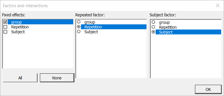
Note: A factor cannot be the subject or repeated factor and a fixed effect at the same time.
Once you have clicked on the OK button, the computation starts. The results will then be displayed.
Interpreting the results of a repeated measures ANOVA
The first results displayed by XLSTAT are the basic statistics associated to the dependent variable.

For each measure, an ANOVA is performed. Results associated to time 0, 1, 3 and 6 are displayed. For more details, you can check the tutorial on one-way ANOVA.
The analysis of variance table pre-test (dv0) is:

The analysis of variance table one month post-test (dv1) is:

The analysis of variance table 3 months follow-up (dv3) is:

The analysis of variance table 6 months follow-up (dv0) is:

We can see that the group has an effect significantly greater than 0 on the depression score after 1 month of treatment.
Once the four analyses have been performed, some additional outputs related to the repeated design are displayed.
The first table is very important and helps to validate the sphericity of the covariance matrix of the errors. This test is called Mauchly’s test.

Given that the p-value is smaller than 0.05 (alpha) we can reject the null hypothesis and accept the alternative hypothesis that the the covariance matrix is not spherical. The Greenhouse-Geisser and the Huynt-Feldt corrections have been applied here to adjust the p-value. Each of these corrections estimate a statistic called espilon. The closer it is to one, the more spherical the covariance matrix is.


The two following tables can now be analyzed. First, the tests on the inter-subject effects which show the effect of the group variable on the whole dataset without taking into account the repetitions (or measures). We see that the group has a significant impact on the depression score. Then, the tests on the intra-subject effects show the impact of time (of the different measures) on the dependent variable. It can be useful to look at the interaction terms between repetition and the explanatory factors. We see that the repetition factor has a significant impact on the depression score; the interaction has also a significant impact.
This study has shown that both time and treatment have a significant impact on the depression score.
Some other outputs can be useful and are available in XLSTAT: residuals, residuals charts, least square means charts, multiple means comparisons...
Was this article useful?
- Yes
- No