Performance indicators for prediction models in Excel

This tutorial shows you how to compare different predictive models with Excel using XLSTAT software.

Dataset for computing modeling performance indicators

The dataset named abalone contains characteristics of abalones, marine gastropod mollusks. To predict the age of an abalone, one needs to color the rings and count them through a microscope, which is a time consuming task. That is why we want to try to predict the age of abalones with measures which are easier to obtain.

After performing two predictive models — SVR (Support Vector Regression) and CART (Classification and Regression Trees — we will try to select the one that will allow us to best predict the age of abalone from their physical characteristics.

Setting up the dialog box for modeling performance indicators

Once XLSTAT is open, click on Model performance Indicators as show below:

The Model performance Indicators dialog box appears.

In the General tab, select the response, which here corresponds to the variable "Rings". In the predicted field, select the predictions (SVR-Pred and TREE-Pred) made with the different models used. Then we check the explanatory variables option to specify the number of variables used in the construction of our models. This information is useful for the calculation of some indicators (adjusted R², AIC, SBC). Here, all the variables (8) in the dataset were used.

The Variable labels option is selected because the first row of the chosen columns contains the names of the variables.

In the Outputs tab, several indicators are proposed, select the ones you want to display.

Interpreting performance indicators for predictive models

The first table provides at a glance the values of the selected indicators for each model.

Error measures such as the RMSE show us that the second model performs better. In order to determine if this difference is large, we can look at the R2, which is an indicator between 0 and 1. It corresponds to the determination coefficient of the model and is interpreted as the proportion of the variability of the response variable explained by the model. The nearer R² is to 1, the better the model is. In our case, about 57% of the variability is explained by the model using the SVR, compared with 40% for the second model.

The adjusted R² is 0.49 for the model using SVR and 0.28 for the one using regression trees.
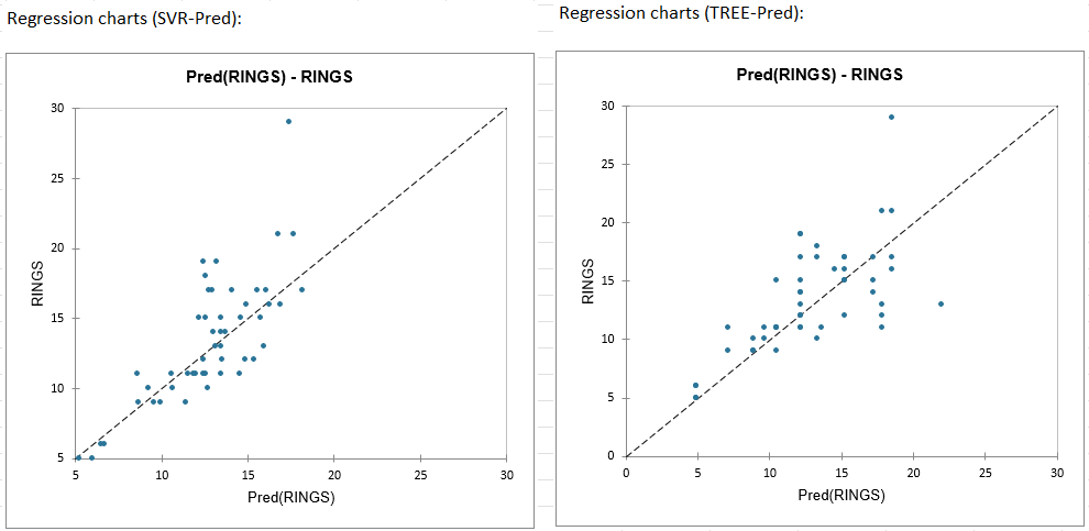
Before looking at the predictions and residuals, let's first have a look on the regression charts. Several charts are displayed for each of the models, but we will focus on 2 of them in this tutorial.

1. Response variable vs Predictions: This chart allows you to compare the predictions and the observed values. The greater the variance explained by the model, the closer the points will be to the regression line.

2. Response variable VS Standardized residuals:

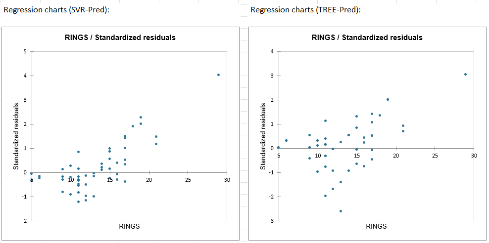
Looking at these graphics, we notice:

• A larger variability of errors on the model using regression trees than for predictions made with the SVR model.

• Good performance (small residuals) of the SVR model on the youngest abalones (RINGS <= 15) and poorer performance for the oldest.

• The existence of an isolated observation (top right). This observation corresponds to the oldest abalone (RING = 29). The table of predictions and residuals will allow us to look at this observation in more detail.

In general, the closer the residuals are to 0, the better the model fits the data.

The following table shows part of the analysis of the predictions and residuals.

In the Residuals column, the residuals with the smallest (resp. largest) deviation from 0 are marked in green (resp. red). This allows us to see for each observation which ones are the best (resp. worst) predicted.

Observation 32 (Obs32) is the one for which the difference between the predicted and the observed value is the largest for the 2 models. It also corresponds to the oldest abalone in our data.

A closer look at this observation shows that it corresponds to the isolated observation in Figure 2 (Response Variable VS Standardized Residuals) and the associated residual is detected as atypical. A residual is marked as atypical if it is significantly higher than the other residues. Thus the predictions associated with this observation should be treated with caution.

Conclusion

In conclusion, the best model among the two compared here is the one using SVR (Support Vector Regression). The model explains 57% of the variability of the age of abalone, and it presents a better distribution of errors than the second model used. However, it is certainly not the most suitable model to predict the age of abalones, because it performs poorly when the age of the abalones is higher than 15. The best solution in our case would be either to combine our SVR model with a second model or to try to build a new model that will be more efficient in predicting the age of abalones.