Multinomial logit model in Excel tutorial

This tutorial will help you set up and interpret a Multinomial Logit regression in Excel using the XLSTAT software. Not sure this is the modeling feature you are looking for? Check out this guide.

What is a multinomial logit model?

The multinomial logit model is a generalization of the classical logit model for variables with more than two modalities to be explained (this method can also be called polytomous logistic regression).

The principle of this model is as follows: we want to understand or predict the effect of one or more variables on a qualitative variable with multiple responses. This variable must be an unordered categorical variable. All the calculations are made relatively to a reference modality that the user must select. This will help us understand the impact of the choice of a modality according to the explanatory variables in relation to a fixed one.

The multinomial logit model is used to model the probability of an event occurring given the values of a set of quantitative and/or qualitative descriptive variables.

Dataset for running a multinomial logit model in XLSTAT

The dataset we use comes from the book "multivariate interpretation of clinical laboratory data" by Adelin Albert and Eugene K. Harris. This data set contains 218 observations from patients with liver diseases (Plomteux, 1980).

The patients were split into four groups corresponding to four types of liver diseases: - Acute Viral Hepatitis (group 1: 57 patients);

• Chronic Persistent Hepatitis (group 2: 44 patients);
• Aggressive Chronic Hepatitis (group 3: 40 patients);
• Post-necrotic Cirrhosis (group 4: 77 patients).

The diagnosis was based on four liver enzymes (U/L): - aspartate aminotransferase (X1: abbreviates AST);

• alanine aminotransferase (X2: ALT);
• glutamate dehydrogenase (X3: GLDH);
• and ornithine carbonyltransferase (X4: OCT).

The diagnosis of acute viral hepatitis was based on classical clinic-biological signs while all other patients were diagnosed following laparoscopy and biopsy findings.

Goal of this multinomial logit model

In our example, we want to predict the probability that a patient has one of the four diseases. The variable to be explained includes four modalities (groups) corresponding to the four diseases.

Setting up a multinomial logit model

To activate the multinomial logit model dialog box, start XLSTAT, then select XLSTAT / Modeling data / Logistic regression.

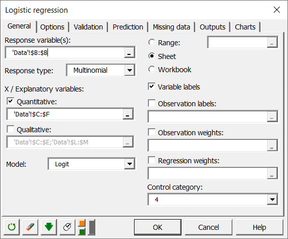
Once you have clicked the button, the dialog box appears. The multinomial logit model is activated by selecting the multinomial option as the response type.

Select the data on the Excel sheet. The Response data corresponds to the column in which the variable to be explained is located, in this case the Group column.

In this example, there are four quantitative explanatory variables corresponding to the four enzymes AST, ALT, GLDH, OCT.

As we have selected the labels of the variables, we must activate the option Variable labels.

We select Modality 4 as the control modality. This does not influence the calculations and predictions, but only the way the equations of the model are written. Many other options are available in the remaining tabs of the dialog box (for more details, see the XLSTAT Help).

Once you have clicked on the OK button, the calculations start and the results are displayed.

Interpret the results of a multinomial logit model

The goodness-of-fit statistics table gives several indicators of the quality of the model. These results are equivalent to the R² in linear regression and to the ANOVA table. The most important value is the Chi² associated with the Log ratio (L.R.). It is the equivalent of Fisher's F-test of the linear model: we try to evaluate if the variables provide a significant amount of information to explain the variability of the response variable. In our case, as the probability is lower than 0.0001, we may conclude that the variables bring a significant amount of information. Next, the Type II analysis table gives the first details regarding the model. It is useful for evaluating the contribution of the variables to the explanation of the response variable. 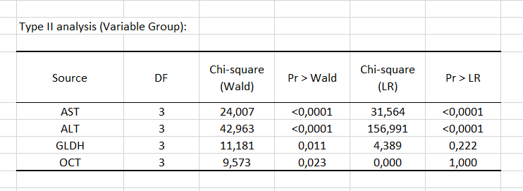According to the probability associated with the Chi-square tests, the variables that most influence the choice of group are the liver enzymes AST and ALT.

The table of model parameters then allows us to test not each variable globally, but its influence on each of the modalities in comparison with the reference one (here 4). Thus, we see that compared to the reference modality, modalities 2 and 3 are influenced by the GLDH variable, because the coefficient is significant (respectively 0.048 and 0.018), which is not the case for modality 1 (0.756). In addition, having a high GLDH value influences having a higher chance of having disease 3 compared to 4 (as the coefficient is positive, 0.058, and the pvalue significant, 0.018).

Next, you can view the Predictions and Residuals table. We see that the fourth observation is associated with group 1, but the model predicts that it should belong to group 2. Indeed, the probability of being in group 2 is the most important and is estimated at 0.443 while the probability of being in group 1, 3 and 4 is estimated at 0.122, 0.131 and 0.304 respectively.

The column Significant change indicates whether the difference between the probability of the predicted group and the one of the actual group is significant. The last column Significant shows if the probability of the predicted group is significantly different from the estimated probabilities for the rest of the groups (modalities). For example, at the 18th observation, the change is significant and the estimated probability for group 2 (0.667) is significantly higher than that of the other groups (0.304, 0.019 and 0.011).

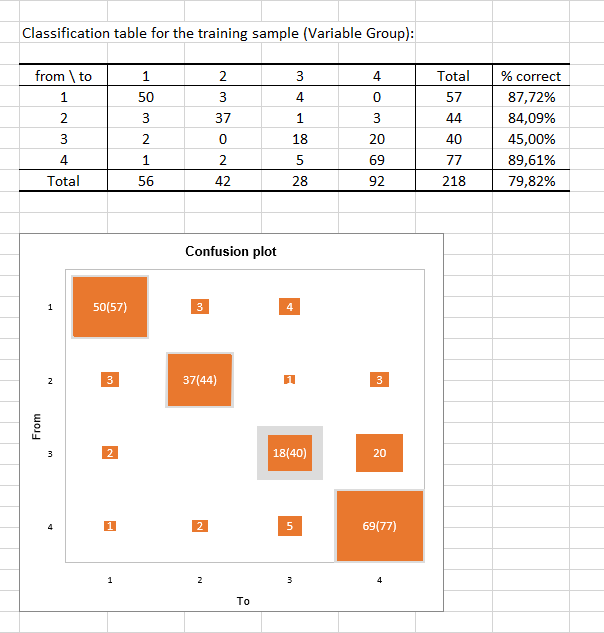
Note that these two columns appear if the Significance analysis option has been checked in the "Outputs" tab of the dialog box. The classification table for the training sample (also called the confusion matrix) shows the percentage of observations that are well classified for each modality (true positives and true negatives). For example, the observations of modalities 1, 2 and 4 were respectively well classified at 87.72%, 84.09% and 89.61% while the observations of modality 3 were well classified for only 45% of the cases.

The confusion plot visualizes the above table in a synthetic way. The grey squares on the diagonal represent the actual observations for each modality. The orange squares represent the predicted observations for each modality. We can see that the surfaces of the squares overlap almost completely for modality 1 (50 predicted observations out of 57 observed observations), modality 2 (37 predicted observations out of 44 observed observations) and modality 4 (69 predicted observations out of 77 observed observations) contrary to modality 3 (18 predicted observations out of 40 observed observations). Finally, the last two tables consider the uncertainty. The first table shows that for 12 observations, the starting value is modality 3, the prediction value is modality 4 and the significance is "Yes" (see the table Predictions and residuals to find these numbers). In other words, there are 12 observations for which the predicted modality is significant.

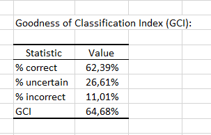
About half (52.50%) of the values predicted by the model for modality 3 can be considered as uncertain, while in the case of modality 1 the values predicted by the model are the least uncertain since the percentage of uncertainty is estimated at 12.28%. 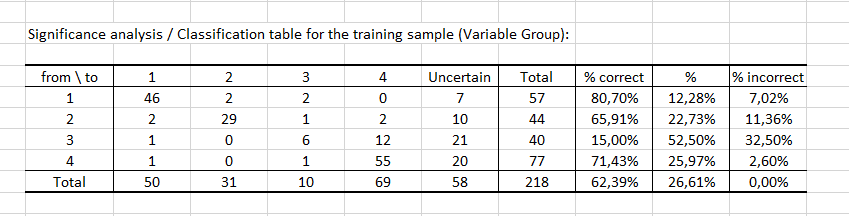Finally, the last table indicates that 62.39% of the observations were well classified (true positives), 26.61% had an uncertain classification and 11.01% were misclassified (false positives and false negatives). The GCI (Goodness of Classification Index) is 64.68%, which means that the predictive quality of this classification model is satisfactory.