Lasso & Ridge regression in Excel
This tutorial will help you set up and interpret a Lasso and a Ridge regression in Excel using the XLSTAT-R engine in Excel.
What are Ridge & Lasso regressions?
In regression cases where the number of predictors is very high, Ridge and Lasso regression techniques have been proposed to provide more accurate coefficient estimations compared to standard techniques. Ridge and Lasso add a regularization term to the regression’s cost function. This term penalizes the cost function as the sum of absolute values of coefficients increase. In Lasso, this term is called L1 Norm and is proportional to the sum of the normed coefficients (sum of |beta|), whereas in Ridge, the term is also referred to as L2 Norm or Thikhonov regularization and is proportional to the sum of the squared coefficients (sum of ||beta||²).
While Ridge regression only tends to shrink coefficients toward zero without setting them to zero, Lasso may, in addition, push some coefficients to become null.
An intermediate technique called Elastic Net has also been proposed to overcome some of the limitations of each of Lasso and Ridge regularizations. Regularization can be controlled using a tuning parameter called Lambda. Regularization strength increases with lambda.
In Machine Learning, Lasso and Ridge regularization are also called weight decay techniques. Ridge, Lasso, and Elastic Net can all be used in cases where the number of predictors is higher than the number of observations or cases.
The Ridge/Lasso/Elasticnet function developed in XLSTAT-R calls the glmnet function from the glmnet package in R (Jerome Friedman, Trevor Hastie, Noah Simon, Junyang Qian, Rob Tibshirani).
Data set for launching a Ridge & Lasso regression in XLSTAT-R
The data were simulated and correspond to 36 biological samples of diseased and healthy individuals belonging to three different genotypes. For each sample, the expression of 1561 genes is measured through RNA quantification. More details are available here. For a better readability of coefficients in the results, it is recommended to label binary outcomes as 0 and 1. Here, healthy patients are labeled 0 and diseased patients are labeled 1.
The goal here is to identify genes which most likely influence the Healthy-Diseased binomial outcome. This is equivalent to investigating differential expression. We will use Lasso regression followed by Ridge regression and compare the outcomes.
Logistic regression cannot be performed here because the number of variables (genes) is far higher than the number of observations (samples).
Setting up a Lasso regression in XLSTAT-R
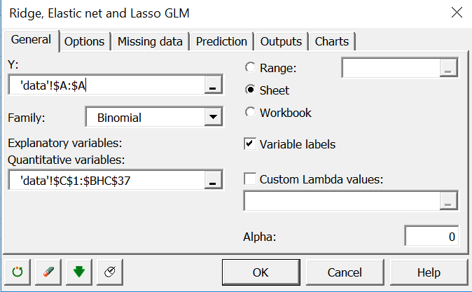
Open XLSTAT-R / glmnet / Ridge, Elastic net and Lasso GLM(glmnet)
 In the general tab, select the status variable (healthy/diseased) in the Y field.
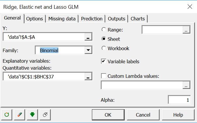 The response is binary. Thus, select the Binomial family. Select all the expression data under the Explanatory quantitative variables field. The alpha parameter controls which type of penalization to apply. Zero is Ridge, one is Lasso and in between is Elastic Net. Set it to 1 for now.
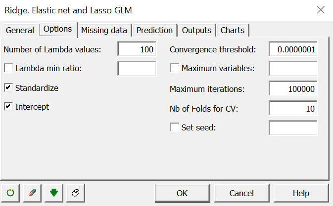
In the options tab, make sure you activate standardize in order to apply data standardization.
Set the number of Lambda values to 100. R will run one model per lambda and use k-fold Cross-Validation to look for an optimal value of lambda among these 100 values.
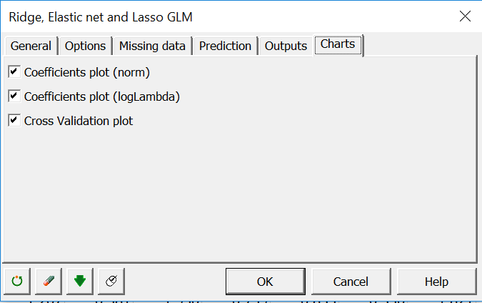
 Activate all charts in the Charts tab.
 Click OK to run the analysis.
Interpretation of a Lasso regression output
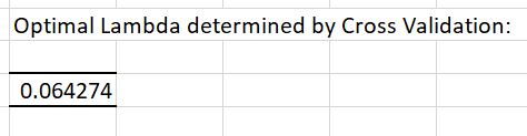
First, the value of Lambda which minimizes deviance is displayed:
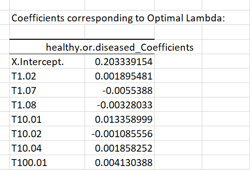
 This is followed by the corresponding computed coefficients for all genes:
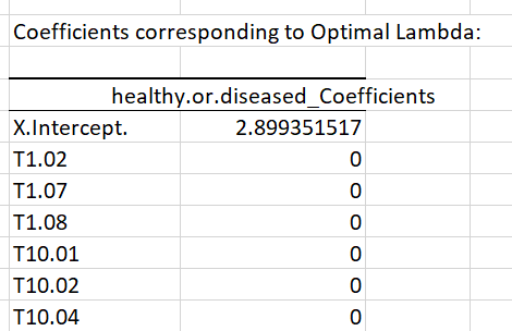
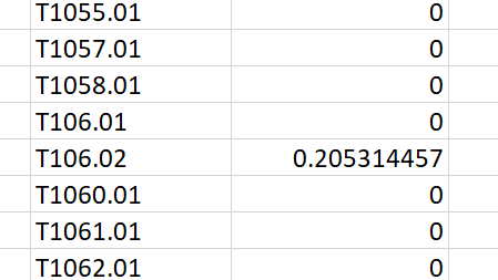
The Lasso penalization set most coefficients to zeros. This helps to determine which features are the most consistent, such as T106.02. As we are running a regression with a binary outcome, coefficients should be interpreted in terms of log-odds. The positive sign reflects the fact that the T106.02 gene seems to be more expressed in diseased patients (recall that diseased patients are labeled as 1 in the data).
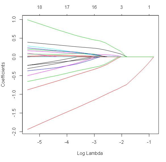
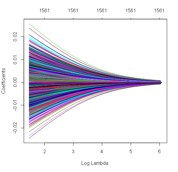
 The Coefficients plot with Log Lambda on the X axis shows coefficient decay as the penalization term Lambda (or its logarithm) increases. Many coefficients end up being null at high values of lambda. Numbers at the top of the chart are the numbers of remaining coefficients at the corresponding Log lambda values.
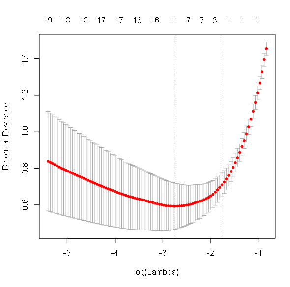
 The Cross Validation plot shows cross validation deviance (or error) according to lambda values. The optimal lambda corresponds to the lambda value at the minimum of this function. Note that the logarithm used for lambda here is the Neperian or natural logarithm.
 Let’s compare these outputs to the outputs of a Ridge regression.
Setting up a Ridge regression in XLSTAT-R
Go back to the glmnet dialog box and set alpha to 0.
 Click OK.
Interpretation of a Ridge regression output
 In opposition to Lasso regression, Ridge regression has attributed a non-null coefficient to each feature. However, these coefficients have been shrunk toward zero. Shrinkage strength increases with the regularization parameter Lambda. This can be seen in the coefficients plot:
¿Ha sido útil este artículo?
- Sí
- No