Three-way ANOVA on a grouped data table in Excel

This tutorial will help you run and interpret a three-way Analysis of Variance (ANOVA) using a grouped data table in Excel with XLSTAT.

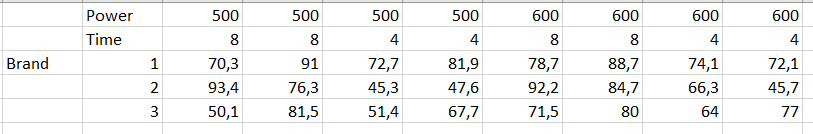
Dataset for running a three-way ANOVA in XLSTAT

The data correspond to an experiment in which three types of microwaves were tested to explain the percentage of edible popcorn after cooking. The cooking differs according to the brand of the microwave, the power, and the time.

Setting up a three-way ANOVA in XLSTAT

• After opening XLSTAT, select the XLSTAT / Modeling / ANOVA feature.

• The ANOVA dialog box appears.

• In XLSTAT, it is possible to select the data in two different ways for a three-way ANOVA. The first one, in the form of columns, requires one column for the dependent variable, and three others for the explanatory variables.

• Select the data on the Excel sheet. The dependent variable corresponds to edible popcorns (%) whose variability we want to explain by the factors brand, power, time as well as their interactions.

• Activate the option Variable labels since the column headers were selected.

• The second way of selecting the data (grouped data table) requires to enter in columns the modalities of two of the explanatory variables, and in rows, the modalities of the third explanatory variable.

• In the Options tab, activate the interactions and set the maximum level of interaction to 2.

• We left the constraint option at a1=0, meaning that the model will be built under the assumption that the brand 1, the power of 500W, and the time of 8 minutes will have the standard effect.

• Applying a constraint to the ANOVA model is necessary for theoretical reasons, but it has no effect on the results (goodness of fit, predictions). The only difference it makes is in the way the model will be written.

• In the Outputs tab, the Type SS options were activated because so that the model takes the interactions into account and so that we can analyze the F values given in the Type I SS, and Type III SS tables (SS stands for sum of squares).

• Once you have clicked the OK button, a dialog box is displayed so that the user can confirm which factors should be included in the model.

• The ANOVA calculations are then performed, and the results are displayed.

Interpreting the results of a three-way ANOVA with interactions

The first table provides the goodness of fit statistics. In our case, 70% of the variability is explained by the brand, the power, the duration and their interactions. The remaining 30% of variability are included in the random part of the model.

The analysis of variance table needs to be analyzed carefully (see below). The results enable us to determine whether or not the explanatory variables bring significant information (null hypothesis H0) to the model. In other words, it's a way of asking yourself whether it is valid to use the mean to describe the whole population, or whether the information brought by the explanatory variables is of value or not.

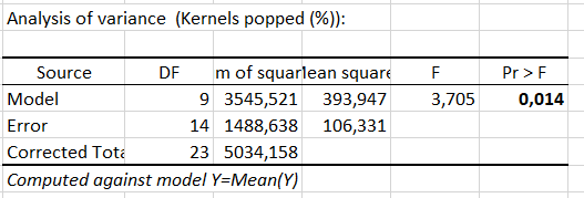
Given that the probability associated with the F is 0.014, it means that we would be taking a 1.4% risk in assuming that the null hypothesis (no effect of the two explanatory variables and their interaction) is wrong. Therefore, we can conclude that the three variables and their interactions do have a significant effect. We also want to find out if the two variables, and their interaction, provide the same amount of information. To do this, we have to examine the Type I SS and Type III SS tables.

The Type I SS table is constructed by adding variables in the model one by one, and by evaluating the impact of each on the model sum of squares (Model SS). In consequence, in Type I SS, the order in which the variables are selected will influence the results.

The Type III SS table is computed by removing one variable of the model at a time to evaluate its impact on the quality of the model. This means that the order in which the variables are selected will not have any effect on the values in the Type III SS.

The Type III SS is generally the best method to use to interpret results when an interaction is part of the model.

Note: the higher the Model SS, the lower the Residual SS, and therefore the greater the influence of the variable.

From the Type III SS table, we can see that Time is the variable which brings the most information to the model. By analyzing the parameters of the model (see below) it can be seen that cooking for 8 minutes has a positive effect on the percentage of edible popcorns. The interaction between brand and duration also has a significant effect, unlike other variables. For the next analyzes, the two main variables will have to be kept.

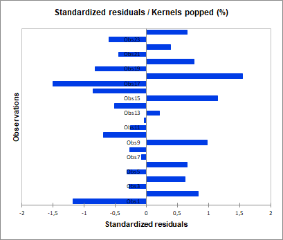
Finally, we can also look at the standardized residuals. These are residuals that, given the assumptions of the ANOVA model, should be normally distributed; i.e., 95 percent of the residuals should be in the interval [-1.96, 1.96]. All values outside this interval are potential outliers or might suggest that the normality assumption is wrong. It appears here that there is no outlier, as all values are in the one [-1.96, 1.96] range.