Random components mixed model in Excel tutorial
This tutorial will help you set up and interpret a random components mixed model in Excel with the XLSTAT software.
Dataset for running a random components mixed model
We use a dataset coming from Mendenhall, Wackerly and Schaeffer (1996, Mathematical Statistics with Applications, Duxbury Press). In this example, ingots made up of various metals are studied. We seek to know the impact of the treated ingot and the type of metal being used as bond in this ingot (N: nickel, I: iron and C: copper) on the necessary pressure to break it into two. We have 7 ingots, three types of bonds and a dependent variable. The treated ingots are drawn from a larger population and thus constitute a random factor in our model.
A mixed linear model is based on the same model as a traditional linear model with a term associated with the random effects. The model will have the following form: ![]()
In our case, Y is the press variable, X is the bond (fixed factor) and Z is the ingot (random factor). Moreover, we can choose the structure of the covariance matrix of the random effects. We will choose a structure called “variance component” which is based on a diagonal matrix. Please consult the help of XLSTAT for more details on covariance structure.
Setting up a random components mixed model
-
After opening XLSTAT, select the XLSTAT / Modeling data / Mixed models command, or click on the corresponding button of the Modeling data toolbar (see below).
-
Select the data on the Excel sheet.
-
The Dependent variable (or variable to model) is here the "pressure". Our aim is to determine the effect of the bond and of the ingot on the variability of the pressure.
-
As we selected the column title for the variables, we left the option Variable labels activated.
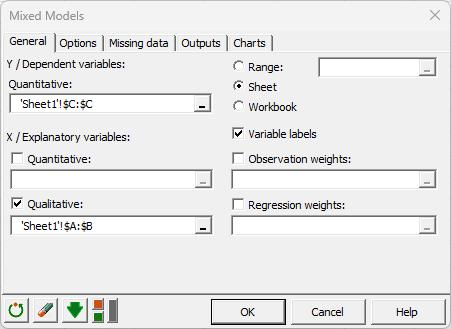
-
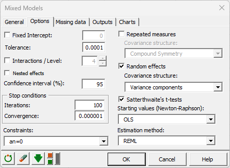
We left the constraint option at an=0, meaning that we want the model to be built on the assumption that the copper has the standard effect on the pressure.
-
When dealing with qualitative variables, although you have to apply a constraint to the model in ANOVA for theoretical reasons, it will not affect the results (goodness of fit). The only difference it makes is in the actual writing of the model.
-
The covariance structure selected is the default one, which is variance component.
-
Once you have clicked on the OK button, a dialog box is displayed so that you can choose which factors have to be taken into account in the model. The fixed effect is the "metal" and the random effect is the "ingots".
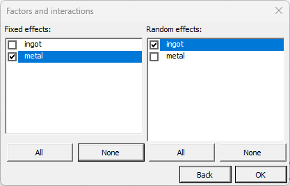
Note: A factor cannot be random and fixed.
-
Once you have clicked on the “OK” button, the computation starts. The results will then be displayed.
Interpreting the results of a random components mixed model
The first results displayed by XLSTAT are the goodness of fit coefficients.
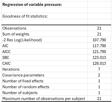
Model parameters are obtained using the restricted maximum likelihood (REML) method and will be different from when a classical linear model is applied. All indexes are used to compare models with different covariance structures.
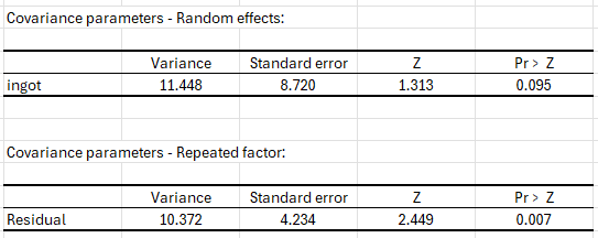
Covariance parameters tables are then displayed. The first one is associated to the random components of the model and the second table is associated to the error covariance matrix. In our case as there is no repeated measures, the error covariance matrix is diagonal with one value associated to the variance.
You can display the full covariance matrix when selecting G matrix (random component covariance) and R matrix (error covariance) in the output dialog box.
We can see that the error variance is significant and the random component variance is not significant. The random component will not have a significant effect on the global model.
To understand the effect of fixed effects on the model, we study the Type III tests of fixed effects. We can see that the metal has a significant effect on the model.
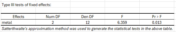
The used metal has a significant effect on the necessary pressure to break the ingot.
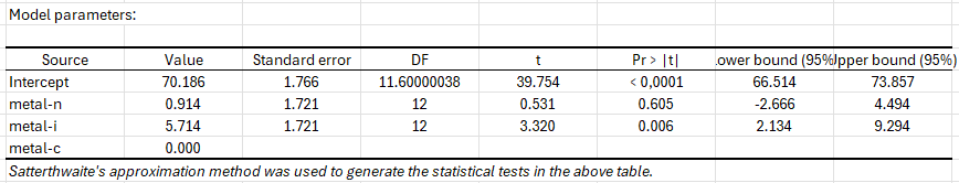
When we look at the model parameters (see below), we can see that using iron as a bond for the ingot makes a significant increase in the necessary pressure. Using nickel does not make a significant difference.
When looking at the random effect coefficients, we can see that all coefficients are not significant and thus conclude that the treated ingot does not affect the model.
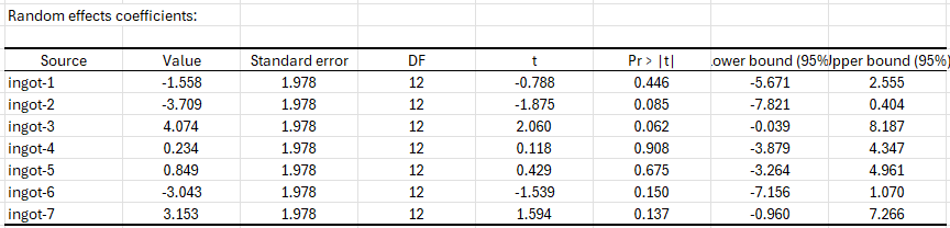
Finally, we can say that the bond is the only factor in the model that has a significant effect on the necessary pressure to break the ingot.
Some other output can be useful and are available in XLSTAT like residuals, residuals charts...
Was this article useful?
- Yes
- No