Customer Long-term Value (CLTV) in Excel tutorial

This tutorial shows how to compute and interpret a Customer Long-term Value analysis in Excel using the XLSTAT software.

Dataset and goal of this tutorial on Customer Long-term Value (CLTV)

The dataset represents a sample of monthly subscription data from a phone service provider. The period covered is from 2010 to 2014. Three groups of users from a value-based segmentation are represented: Young, Classic and Premium. The goal of this tutorial is to calculate the CLTV (customer long-term value) of customers and to obtain a detailed overview of the customers life cycle.

Setting up a Customer Long-term Value dialog box

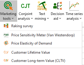
Once XLSTAT is launched, select the Advanced Functions / Marketing Tools / CLTV feature.

The Customer Long-term Value dialog box appears:

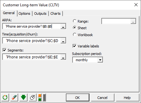
In the General tab, select the column corresponding to the subscription price in the ARPA (Average Revenue Per Account) field. Then select in order the two columns related to the acquisition date and churn date in the field Time(acquisition/churn). Our data set contains segments variable, so check the case Segments and select the corresponding data to allow XLSTAT to produce results by segments.

As the subscriptions are monthly, select monthly in the subscription period field.

In the Options tab, we can take certain parameters, such as the discount rate or fixed operating costs, into account in the CLV computation. The customers being charged at the beginning of the month, we choose the option Start of period in the Payment section.

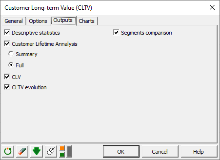
In the Outputs tab, choose the results to display. The segment comparison option allows a comparison of the retention functions between the different segments in order to identify any similarities.

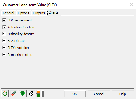
In the Charts tab, we have the choice between several curves to display such as the comparison graphs which allow to display graphs comparing the retention, density and hazard curves for the different segments. This can be useful to get an overview of customers behavior by segment.

The computations begin once you have clicked on OK.

Interpret the results of Customer Long-term Value (CLTV)

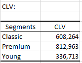
After the descriptive statistics table, the first result displayed is the average CLV per segment.

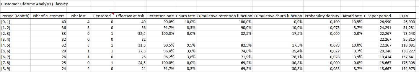
Then, for each segment, we obtain the customer lifetime analysis table. This table gives us a set of statistics on the customers behaviour.

The first columns of the table provide a summary of customers actions. We can therefore observe for each month how many customers have cancelled their subscription, how many customers are no longer being observed (censored) and have the corresponding retention and churn rate.

The cumulative churn function gives us the proportion of lost clients since the beginning of the study. Let's look at the Classic segment, more specifically at the period [5.6] which is the 6th month after subscription. The value of the cumulative churn function is 25.4%. This means that about a quarter of the customers cancelled their subscriptions within the first 6 months following their subscription.

The probability density function gives the probability that a customer is retained during the first t-1 periods and cancels during period t. For the Classic segment, the probability that a customer will cancel his subscription during the 6th month of subscription is 0.027 (2.7%).

The hazard rate is the conditional probability of canceling at time t given that the customer has not never canceled. The probability that a customer in the Classic segment will cancel the membership during the 6th month knowing that he or she was a customer the month before (5th month) is 3.7%.

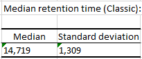
The last two columns display the estimates of CLV (customer lifetime value) and CLTV. We can see that a customer in the Classic segment who cancels the subscription during his 6th month of subscription will have an average CLTV of 138,227€. The median retention time and the associated standard deviation are following. For the classic segment, half of the customers are lost after 15 months (14,719).

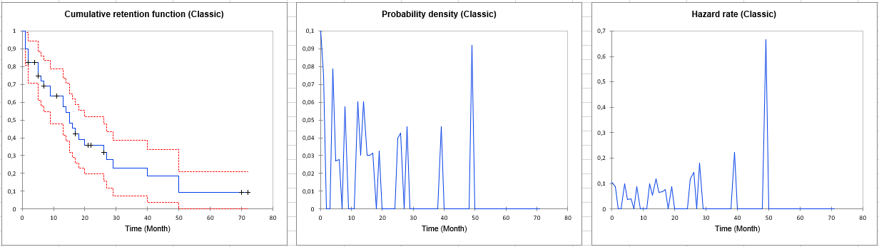
Several charts are generated next which summarize the information contained in the previous tables.

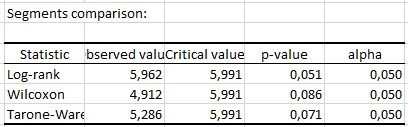
The following output is also displayed since we selected the option Comparison of segments. It contains the results of three different tests: the Log-rank test, the Wilcoxon test, and the Tarone Ware test. These tests are based on a Chi-square test. The lower the p-value, the more significant the differences between the segments.

As we can see in the table below, none of the tests are significant at the threshold alpha = 5%.

There is no significant difference between the retention curves of our 3 segments.

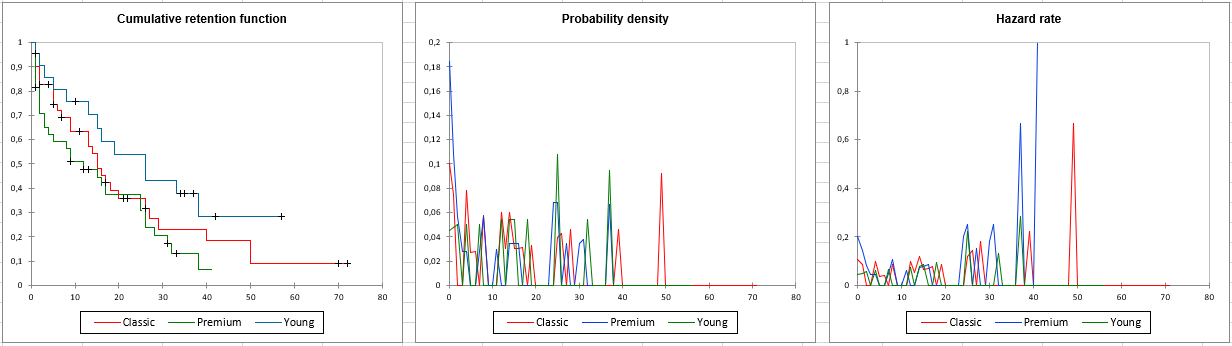
Finally, a chart comparing the retention, density and hazard curves for the different segments is generated.