Consumer satisfaction analysis in Excel with PLSPM
This tutorial shows how to compute and interpret an a consumer satisfaction analysis in a Partial Least Squares Path Modeling context in Excel using the XLSTAT software.
Principles of PLS path modeling
Partial Least Squares Path Modeling (PLS-PM) is a statistical approach for modeling complex multivariable relationships (structural equation models) among observed and latent variables. This family of models is generally called structural equation models with latent variables. PLS-PM seeks for optimal linear predictive relationships rather than for causal mechanisms thus privileging a prediction-relevance oriented discovery process to the statistical testing of causal hypotheses. Two very important review papers on PLS approach to Structural Equation Modeling are Chin (1998, more application oriented) and Tenenhaus et al. (2005, more theory oriented). Latent variable scores estimated using the PLS-PM approach are very useful in computing global indices that include the consumer satisfaction index.
PLS Path Modeling using XLSTAT-PLSPM
In this tutorial we guide you step by step to show you how to create a project, define a model, estimate the parameters and analyze the results in the framework of the analysis of consumer satisfaction. The application is based on real life data, where 250 customers of mobile phone operators have been asked several questions in order be able to model their loyalty. The PLSPM model is based on the European Customer Satisfaction Index (ECSI). In the ECSI model, the latent variables (concepts that cannot be directly measured) are interrelated as displayed below.

Each latent variable is related to one or more manifest variables that are measured. In this application case, the manifest variables questions are on a 0-100 scale. For example, for the Image latent variable the five manifest variables are:
- It can be trusted in what it says and does
- It is stable and firmly established
- It has a social contribution for the society
- It is concerned with customers
- It is innovative and forward looking
An XLSTAT-PLSPM project sheet containing both the data and the results for use in this tutorial can be downloaded.
XLSTAT-PLSPM projects are special Excel workbook templates. When you create a new project, its default name starts with PLSPMBook.
You can then save it to the name you want, but make sure you use the "Save" or "Save as" command of the XLSTAT-PLSPM menu to save it in the folder dedicated to the PLSPM projects using the *.ppmx extension. Furthermore, when you create a project, a dialog box appears asking you to choose the display type. In the satisfaction analysis framework, we will use the Marketing mode which simplifies dialog boxes and outputs.
Note: when you open the PLSPathModeling_ECSI.ppmx file, the graphical representation might look bad. This is due to the fact that the representation depends on your screen settings. To improve the display, click the "Optimize the display" button (see below).
A raw XLSTAT-PLSPM project contains two sheets that cannot be removed: - D1: This sheet is empty and you need to add all the input data that you want to use into that worksheet.
- PLSPMGraph: This sheet is blank and is used to design the model. When you select this sheet, the "Path modeling" menu is displayed on the upper left part of the page.
When you open an existing project, the display mode could be changed anytime by clicking on the XLSTAT-PLSPM options in the PLSPM menu.

In this tutorial, we will focus on the Marketing display that lets you use PLS Path Modeling in consumer satisfaction analysis. Save the project using the Save the project as function. Remark: you should always save and open your .ppmx projects using the PLSPM functions and not the classical Excel functions.
Then, we copied the data that were available in an Excel file, and pasted them into the D1 sheet of the Project. Once this is done, you are ready to start creating the model. Move to the PLSPMGraph sheet. The toolbar is displayed on the upper left corner of that sheet.

To create several latent variables in a row, double click on the circle button so that it stays pressed while you add variables:

You can then add the arrows that indicate how the latent variables are related. To add an arrow, click on the latent variable from which it should start, then press Ctrl and click on the latent variable where the arrow should end. Then click on the arrow button or use the following keyboard shortcut: Ctrl+L.

Another method lets you load predefined models, using the seventh button. You will be able to load the model from a library that already contains a list of famous models. The selected model will be automatically imported in the project. PLSPM Models have a .ppmxmod extension.
Once all the arrows have been added, you can define the manifest variables that relate to each latent variable (this can also be done after adding the latent variables). To add manifest variables to a latent variable, select the latent variable and click on the MV button in the toolbar:

This activates the D1 sheet and displays a dialog box where you give a proper name to the latent variable, select the manifest variables on D1 and define a few settings.
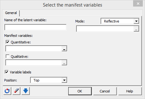
The mode has to be defined. In Mode A (reflective mode) the latent variable is responsible for what is measured for the manifest variables, and in Mode B (formative mode), the manifest variables construct the latent variable. In our example we assume that our manifest and latent variables are linked with mode A.
Here is the dialog box configuration for the expectation latent variable:

The obtained model has the following form:

Once the manifest variables have been defined for each latent variable and latent variables are linked, you can start computing the model. To run the model, click the play button.

This displays the Run dialog box, where many options are available. For this tutorial the following options have been used:
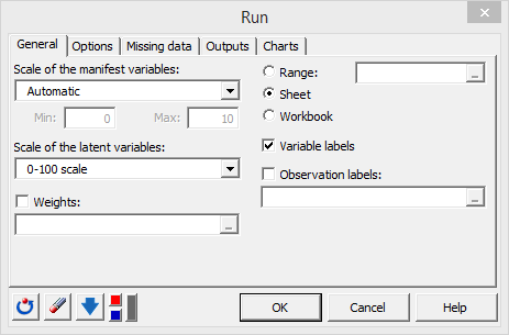
In our example, we use the automatic mode for the scale of the manifest variables and the 0-100 scale for the latent variables. Keep the default Options tab configuration unchanged. Configure the outputs tab as follows:

Activate the Simulation table option and select the Satisfaction latent variable to be explained because we want to study the effects of a change in the model variables on this specific variable. The scale of the change is measured in percentage and spans from -10% to 10% with a step of 1%. Also activate the IPMA table (Important Performance Matrix Analysis).
Results and interpretation of a PLSPM project outputs
The first part of the results gathers information on the data and on the created model (descriptive statistics related to the manifest variables and model specification).
It is first important to check blocs unidimensionality. In our case (reflective variables), blocs must be unidimensional. The Composite reliability table provides this information:
 The Cronbach alpha is below the 0.7 threshold for the Expectation and Loyalty variables. However, Dillon and Goldstein’s rho is above the 0.7 threshold for all variables. Finally, the first eigenvalue is higher than the second in many cases. Those results let us consider that blocs are unidimensional, although it could be interesting to investigate supplementary dimensions in expectation and loyalty. The Complaint latent variable does not appear in the table as it is associated to one single manifest variable.
The next table contains information on the goodness of fit index.
 The absolute GoF = 0.484. It is very close to its bootstrap estimation. This value is not easy to interpret. It is mostly used to compare different groups of individuals or different models. The relative GoF and GoFs based on internal and external models are very high and reflect a likely good fit of the model to the data.
The two following tables display external weights and the correlations associated to the measurement model.
Once the measurement model is studied, the structural model can be analyzed. Each latent variable is associated to several outputs. We will comment the outputs of the satisfaction variable:
 We may consider that the latent variable is well explained (R²=0.681). We see that the perceived quality has the most important effect on satisfaction followed by the perceived value. The expectation impact is insignificant. The last table summarizes the preceding results. We see that the perceived quality has a 59% contribution to the R².
The following chart illustrates the tables we just commented:
We may consider that the latent variable is well explained (R²=0.681). We see that the perceived quality has the most important effect on satisfaction followed by the perceived value. The expectation impact is insignificant. The last table summarizes the preceding results. We see that the perceived quality has a 59% contribution to the R².
The following chart illustrates the tables we just commented:
 Next, outputs linked to the marketing analysis are displayed starting with the IPMA (Importance Performance Matrix Analysis). The IPMA allows to visualize the importance and performance of latent variables on a target variable. Here is the chart for the satisfaction variable:
 We see that quality is the most important and performant latent variable. It will be difficult to increase this variable’s performance since it is already too high. It is followed by the expectation and image variables that share the same importance. Image seems interesting because it has a lower performance and it could be improved more easily than other variables.
Then the simulation charts are displayed. First, for the manifest variables:
The first chart summarizes the effect of a X% increase of a manifest variable on satisfaction. For a 10% change we obtain:
We see that quality is the most important and performant latent variable. It will be difficult to increase this variable’s performance since it is already too high. It is followed by the expectation and image variables that share the same importance. Image seems interesting because it has a lower performance and it could be improved more easily than other variables.
Then the simulation charts are displayed. First, for the manifest variables:
The first chart summarizes the effect of a X% increase of a manifest variable on satisfaction. For a 10% change we obtain:
 The QUALITY5 variable has the strongest effect.
The following chart is the same as the current one but uses the mean value as a base.
Then the changes to the latent variables are investigated:
The QUALITY5 variable has the strongest effect.
The following chart is the same as the current one but uses the mean value as a base.
Then the changes to the latent variables are investigated:
 Here we see that a 10% increase of quality will result in an increase of 17% in satisfaction. The same chart based on means is displayed next.
In the remaining outputs, we find the latent variable scores as well as the associated descriptive statistics. Those scores can be used for other analyses in XLSTAT.
To Conclude
This analysis showed how to investigate a dataset using a satisfaction model. We illustrated the use of the PLS Path Modeling approach lets you easily understand the interactions between concepts. Once the model is validated, it coefficient interpretation and result analysis are very simple.
Was this article useful?
- Yes
- No