Compute sample size and power for a comparison of correlations in Excel

This tutorial explains how to calculate the sample size and power for a comparison of correlations in Excel using XLSTAT.

What is the power of a statistical test?

When testing a hypothesis using a statistical test, there are several decisions to take:

• The null hypothesis H0 and the alternative hypothesis Ha.

• The statistical test to use.

• The type I error also known as alpha. It occurs when one rejects the null hypothesis when it is true. It is set a priori for each test and is 5%.

The type II error or beta is less studied but is of great importance. In fact, it represents the probability that one does not reject the null hypothesis when it is false. We cannot fix it upfront, but based on other parameters of the model we can try to minimize it. The power of a test is calculated as 1-beta1−beta and represents the probability that we reject the null hypothesis when it is false.

We therefore wish to maximize the power of the test. XLSTAT calculates the power (and beta) when other parameters are known. For a given power, it also allows to calculate the sample size that is necessary to reach that power.

The statistical power calculations are usually done before the experiment is conducted. The main application of power calculations is to estimate the number of observations necessary to properly conduct an experiment.

Goal of this tutorial

We want to compare the height-weight correlation for men and women. The goal of this tutorial will be to find the right sample size in order to obtain a power of 0.9. As we do not know yet the parameters of our samples, we will use the concept of effect size. Cohen (1988) introduced this concept which makes it possible to give an order of magnitude for the importance of the effect, the relative difference between the correlations.

We will therefore test 3 effect sizes: 0.1 for a weak effect, 0.3 for a moderate effect and 0.5 for a strong effect. Since the effect size is based on the difference between the correlations, it is expected that the stronger the effect (hence the difference), the smaller the sample size needed.

Setting up the sample size calculation for a comparison of correlations

Once XLSTAT has been launched, click on the Power icon and choose Compare correlations.

Once the button is clicked, the dialog box pops up.

Choose the objective Find the sample size, and as test the Correlations test for two samples. We will take as an alternative hypothesis r1 - r2 <> 0.

The alpha is 0.05, the desired power is 0.9.

We want to have samples of the same size, so we take a ratio N1/N2 equal to 1. Since we don't know the parameters of our samples, we use the effect size, which we choose to set to 0.1.

In the Chart tab, the simulation plot option is activated and the size of sample 1 will be represented on the vertical axis and the power on the horizontal axis.

The power varies between 0.8 and 0.95 in intervals of 0.01.

Once you click on the OK button, the calculations are done and then the results are displayed.

Interpreting the results of sample size calculations for a comparison of correlations

The first table shows the essential results including the sample size followed by an interpretation.

We see that 2104 observations are needed for the two samples to obtain a power as close as possible to 0.9.

The following table gathers the calculations obtained for each value of the power between 0.8 and 0.95.

The simulation plot shows the evolution of the sample size as a function of the power. We see that for a power of 0.8, just over 1573 observations per sample are enough and that for a power of 0.95 we arrive at 2757 observations.

For effect sizes of 0.3 and 0.5, the following results are obtained:

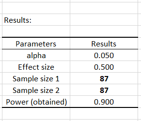
The sample size will therefore decrease because the difference between the correlations increases and we see that for a strong difference, 87 observations per sample will be sufficient.

XLSTAT is a powerful tool both for finding the appropriate sample size and for calculating the power of a test. Obviously, if one has more information about their samples, they can give details of the input parameters, rather than entering the size of the effect.